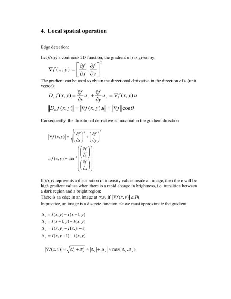
4. Local spatial operation
Edge detection:
Let f(x,y) a continous 2D function, the gradient of f is given by:
 f f 
f ( x , y )   , 
 x y 

The gradient can be used to obtain the directional derivative in the direction of u (unit
vector):
Du f ( x, y ) 
f
f
ux 
u y  f ( x, y ).u
x
y
Du f ( x, y )  f ( x, y ).u  f cos
Consequently, the directional derivative is maximal in the gradient direction
 f   f 
f ( x, y )      
 x   y 
2
2
  f  
   
1   y  
f ( x, y )  tan 
f 
   
  x  


If f(x,y) represents a distribution of intensity values inside an image, then there will be
high gradient values when there is a rapid change in brightness, i.e. transition between
a dark region and a bright region:
There is an edge in an image at (x,y) if f ( x, y)  Th
In practice, an image is a discrete function => we must approximate the gradient
 x  I ( x, y )  I ( x  1, y )
 x  I ( x  1, y )  I ( x, y )
 y  I ( x, y )  I ( x, y  1)
 y  I ( x, y  1)  I ( x, y )
I ( x, y)  2x  2y   x   y  max(  x ,  y )
Gradient edge operators:
 1 0 1
Prewitt:  1 0 1


 1 0 1
 1  1  1
  1 0 1
 0 0 0  Sobel:  2 0 2




 1 1 1 
  1 0 1
Kirch (a directional operator):
3 3  5
3  5  5
3 0  5
3 0
5  …



3 3  5
3 3
3 
 1  2  1
0
0
0 

 1
2
1 
Original image
Sobel (magnitude)
The Canny edge detector:
1. Compute I ( x, y )
2. Suppress any edge that is not a local maximum in the gradient direction (nonmaximal suppression)
3. Use two thresholds Tlow and Thigh (hysteresis thresholding); keep only edge points
where I ( x, y)  Tlow and for which it exists a continuous path of edges linking
that edge point to an edge with I ( x, y )  Thigh . Consequently, all ‘ Thigh ’ edge
points are kept while all chains of ‘ Tlow ’ edge points that do not touch a ‘ Thigh ’
edge point are removed.
Tlow= 1 Thigh=255
Sigma= 1.0, Tlow= 220 Thigh=255
Sigma= 1.0, Tlow= 1 Thigh=128
From : http://www.cee.hw.ac.uk/hipr/html/canny.html
The Laplacian:
2 f 2 f
 f ( x, y ) 

x 2
y 2
2
which can be approximated by:
1 1 1
0 1 0 
1  8 1 or 1  4 1




1 1 1
0 1 0
The contours of an image can be enhanced by the following transformation:
I enhanced( x, y )  I ( x, y )   2 I ( x, y )
http://micro.magnet.fsu.edu/primer/java/digitalimaging/processing/kernelmaskoperation/
The edges of an image are located at the zero-crossings of the Laplacian.
Advantages: no thresholds, subpixel localization.
Problem: very sensitive to noise. Solution: to smooth the image before.
Image smoothing (noise reduction):
Images are often corrupted by (additive) noise
I noisy ( x, y )  I ( x, y )  n( x, y )
2 types of noise:
o Gaussian noise: the noise is Gaussian distributed with zero-mean and a
given variance.
G ( x) 
1
2 

e
x2
2 2
o Salt and pepper noise: some pixel values are lost (they are replaces by
black or white dots)
1 1 1
1
ean filter: 1 1 1
9
1 1 1
5x5 mean filter
Minimal mean square error filter:
I filtered ( x, y)  I ( x, y) 
2
 noise
2
 neighborho
od
[ I ( x, y)  I ( x, y)]
Median filter: replacing the current pixel value by the middle-ranked value of a
neighborhood of predefined size.
5x5 median filter
Gaussian filter: use a Gaussian mask
G ( x, y ) 
1
2 2
1
4
7
4
1
4
16
26
16
4
7
26
41
26
7
4
16
26
16
4
1
4
7
4
1
______
273

e
x2  y 2
2 2
Gaussian filter
Computing image derivative using Gaussian kernels
Applying a Gaussian mask:
I filtered ( x, y )   I ( x  i, y  j )G (i, j )   I (i, j )G ( x  i, y  j )
i, j
i, j
First derivative: applying the following mask correspond to smooth the image and then
derivate it with respect to x.

G ( x, y )
x

e
x
2 4
x2  y2
2 2
The Laplacian of Gaussian: applying the following mask correspond to smooth the image
and then compute the Laplacien.
LoG ( x, y )  
1

[1 
4
x y
]e
2 2
2
2

x2  y2
2 2
sigma=1.4
Difference of Gaussian:
provide an approximation to the LoG
from http://www.cs.toronto.edu/~jepson/csc2503/tutSIFT04.pdf
from: P.J. Burt, E.H. Adelson The Laplacian as a compact image code, IEEE trans. on Comm.-32, no 4, April 1983.
Interest point detection
Goal: to identify feature points that be accurately localized in an image.
Corners are useful features that can be accurately detected in an image. They are often
used for tracking and matching.
 The Harris corner detector:
The average change of intensity in direction (u,v) is given by (Taylor expansion):
2
  I 2  I 2


I
I
I I 
2
R   I ( x  u, y  v)  I ( x, y)     I ( x, y)  u  v  I ( x, y)      u    v   2
uv
  x   y 
x
y
x y 




which can be rewritten as:
u 
R  u v C  
v 
  I  2
  
 x 
C
 I I

 x y
I I 
 x y  a b

2  

 I   b c 
  y  
  
Now if, for a given pixel, we find the direction for which R is maximal and if that R is
high and if the R in the perpendicular direction is also high, then we have a corner.
Corners are found by extracting the eigenvalues and eigenvectors of this matrix:

  0.5 a  c   4b 2  a  c 

There will be a corner if min 1 , 2  is greater than a predefined threshold.
2
“Edge”
2 >> 1
“Flat”
region
“Corner”
1 and 2 are large,
“Edge”
1 >> 2
1
Feature matching:
http://www.cs.washington.edu/education/courses/cse576/08sp/lectures/features.ppt.
Epipolar geometry:
http://www.computerrobotvision.org/2010/tutorial_day/crv10_epipolar_laganiere.pdf
 The FAST corner detector:
A simple corner detector that detects interest points based on local intensity values.
768 x 288 pixels => 2.6ms versus 44ms for Harris
Principle: a circle of pixels surrounding a candidate point is examined. A feature is
detected at the center point if a sequence of contiguous points of length greater than 75%
of the circle perimeter are all above or below the intensity of the center point by some
threshold.
Candidates can be rejected quickly by testing four points (up, down, left, right).
from: Edward Rosten and Tom Drummond, October 2005, IEEE International Conference on Computer Vision
Feature points can be matched using Variance Normalized Correlation:
 The SIFT features (David Lowe, UBC):
What is the LoG response to a corner?
from: S. Tabbone, L. Alonso and D. Ziou, Behavior of the LoG extrema, Int. Journal of Mathematical Imaging and Vision, 2005
Interest points correspond to local extrema of difference-of-Gaussian filters at  and k
from: http://www.cs.ubc.ca/~lowe/keypoints/
 A window of size proportional to  is extracted.
 The dominant orientation of the gradient vectors inside the window defines the
orientation of the feature.
from: http://www.cs.ubc.ca/spider/lowe/papers/iccv99.pdf

SIFT feature descriptor: made of histograms of orientations, each of them made of 8
bins. When 16 histograms are used, a vector of 128 elements is obtained that is then
normalized to enhance invariance to illumination changes.

Feature are matched by measuring the distance between the descriptor vectors of
keypoints. For robustness, use ratio of nearest neighbor to ratio of second nearest
neighbor.

Recognition using SIFT features
o
o
o
o
Compute SIFT features on the input image
Match these features to the SIFT feature database
Each keypoint specifies 4 parameters: 2D location, scale, and orientation.
To increase recognition robustness:
 Hough transform to identify clusters of matches that vote for the same
object pose.
 Each keypoint votes for the set of object poses that are consistent with the
keypoint's location, scale, and orientation.
 Locations in the Hough accumulator that accumulate at least 3 votes are
selected as candidate object/pose matches.
 A verification step matches the training image for the hypothesized
object/pose to the image using a least-squares to the hypothesized location,
scale, and orientation of the object.
from: http://www.cs.toronto.edu/~jepson/csc2503/tutSIFT04.pdf
SURF
This feature detector uses simple masks to approximate second-order derivatives. These
are used to estimate the value of the Hessian:
It is applied at various scales and interest points are found at local maxima.
SURF Descriptor:
BRIEF descriptor
Binary descriptor: differences between random pixel pairs (128 bits)
FREAK descriptor
MSER: Maximally Stable Extremal Regions
With MSER, the image is slowly ‘flooded’ with water and areas that retain their shape for
a sufficiently long period of time becomes features.
Line detection:
Goal: to detect a sequence of points aligned along a straight line.
A. Local edge linking
1. Start from some arbitrary edge point
2. Search for points with similar edge direction in the neighborhood of that point
3. If such similar point is found, add the point to the current set of edges and repeat
search from this point.
B. Gradient partitioning
1. Use a gradient operator to partition the image into edges of different orientations.
For example, the Kirch operator can be used to group the pixels into 8 directions.
2. Group pixels of similar orientation in clusters (connected components).
3. For each group, find the best line that fits the data set.
C. The Hough transform:
Uses the following line representation:   x cos   y sin 



Create an accumulator A(  ,  ) where
o  is quantized between  min and  max by step of 
o  is quantized between  min and  max by step of 
For each 
o compute   x cos   y sin 
o increment A(  ,  )
Lines are found at the local maxima of A(  ,  )
To detect circles, use ( x  a) 2  ( x  b) 2  r and a 3D accumulator A(a,b,r)
There is also a Hough transform for arbitrary shapes.
Example of Hough transform: