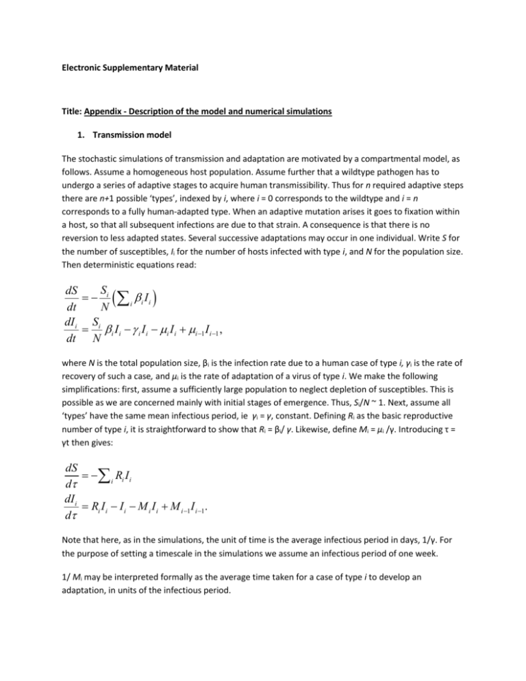
Electronic Supplementary Material
Title: Appendix - Description of the model and numerical simulations
1. Transmission model
The stochastic simulations of transmission and adaptation are motivated by a compartmental model, as
follows. Assume a homogeneous host population. Assume further that a wildtype pathogen has to
undergo a series of adaptive stages to acquire human transmissibility. Thus for n required adaptive steps
there are n+1 possible ‘types’, indexed by i, where i = 0 corresponds to the wildtype and i = n
corresponds to a fully human-adapted type. When an adaptive mutation arises it goes to fixation within
a host, so that all subsequent infections are due to that strain. A consequence is that there is no
reversion to less adapted states. Several successive adaptations may occur in one individual. Write S for
the number of susceptibles, Ii for the number of hosts infected with type i, and N for the population size.
Then deterministic equations read:


S
dS
  i  i i Ii
dt
N
dI i Si
 i I i   i I i  i I i  i 1 I i 1 ,
dt N
where N is the total population size, βi is the infection rate due to a human case of type i, γi is the rate of
recovery of such a case, and μi is the rate of adaptation of a virus of type i. We make the following
simplifications: first, assume a sufficiently large population to neglect depletion of susceptibles. This is
possible as we are concerned mainly with initial stages of emergence. Thus, Si/N ~ 1. Next, assume all
‘types’ have the same mean infectious period, ie γi = γ, constant. Defining Ri as the basic reproductive
number of type i, it is straightforward to show that Ri = βi/ γ. Likewise, define Mi = μi /γ. Introducing τ =
γt then gives:
dS
  i Ri I i
d
dI i
 Ri I i  I i  M i I i  M i 1I i 1.
d
Note that here, as in the simulations, the unit of time is the average infectious period in days, 1/γ. For
the purpose of setting a timescale in the simulations we assume an infectious period of one week.
1/ Mi may be interpreted formally as the average time taken for a case of type i to develop an
adaptation, in units of the infectious period.
2. Simulation
The system described above is translated into a stochastic simulation, in continuous time, using the
Gillespie algorithm (18). Given a time τ and a state vector n(τ), whose ith entry is the number of people
infected with strain i at time τ, there are 3P possible next events, where P is the total number of
infecteds at time τ: each infected can, as above, transmit, recover, or develop an adaptation. With each
possible event we associate a ‘weight’, as follows:
R0(i)
(Transmission from an individual infected with strain i)
1
(Recovery of an individual infected with strain i)
M(i)
(Mutation in an individual infected with strain i)
so that the sum of these weights over all individuals is s = ∑i ni(R0(i)+1+Mi). Dividing each of the weights by
s, we find the next-event-probabilities for each of the above described events. Generating a uniformly
distributed random number between 0 and 1 determines which of these events happen next, and to
which individual: the time to this event is given by c = – log(r)/s, where r is a second random number
uniformly distributed between 0 and 1. Thus we obtain an updated state vector, n(τ + c).
Given an index human case of a wildtype pathogen, the above process is repeated until there are zero
remaining infected cases (extinction), or there are sufficiently many cases that the probability of
ultimate extinction is less than 10-6 (emergence). This probability is given by R0-m, for m cases of a
pathogen with R0 > 1. The choice of 10-6 is an arbitrary one; indeed, it may argued that in some cases a
more conservative threshold probability of, say, 0.5 could be adopted. However, even such a relatively
high probability does not materially affect the results presented here: as discussed in the text, large,
self-limiting clusters arise not from adapted strains, but from those marginally below adaptation.
Title: Appendix - Extensions to the model
The results presented in the text assume, for simplicity, that all clusters are due to a single zoonosis. To
simply model the effect of multiple introductions in the same cluster, we assume here that the number
n0 of such introductions is a Poisson random variable, conditioned on n0 ≥ 1, that is:
Pr(n0 = k) = λk/[k!(eλ-1)], k ≥ 1.
In the example of H5N1 influenza, an upper bound on λ is given by assuming that all human cases have
been zoonoses. Thus, data from Indonesia (World Health Organization 2009) suggests that λ ≤ 0.14.
Figure A1 shows cluster size distributions before emergence, assuming λ = 0.14. It also incorporates
evolutionary courses involving seven adaptive stages, a greater number than presented in the text.
Despite these modifications, qualitative properties of adaptive and gradual scenarios remain unchanged.
10
Frequency
10
5
10
0
10
0
2
4
6
8
10
10
Frequency
10
5
10
0
10
0
10
20
30
40
50
Cluster size
60
70
80
Figure A1: Simulated cluster size distributions for an ‘extended’ model, incorporating seven adaptive
stages and the possibility of multiple index human cases arising from a single zoonotic host. See
caption, figure 3, for an explanation of these plots. Here the punctuated scenario (upper graph) has R0 =
[0, 0.1, 0.1, 0.1, 0.1, 0.1, 2] and the gradual scenario (lower graph) has R0 = [0, 0.1, 0.3, 0.6, 0.9, 1.4, 2].
Both cases have M = [0.1, 0.1, 0.1, 0.1, 0.1, 0.1, 0].
Video of series of introductions leading to emergence
Description: Animations illustrating the accumulation of outbreaks before emergence of an adapted
virus, for both the punctuated and the gradual scenarios.
(Please see movie file sent separately)