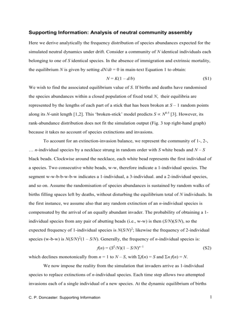
Supporting Information: Analysis of neutral community assembly
Here we derive analytically the frequency distribution of species abundances expected for the
simulated neutral dynamics under drift. Consider a community of N identical individuals each
belonging to one of S identical species. In the absence of immigration and extrinsic mortality,
the equilibrium N is given by setting dN/dt = 0 in main-text Equation 1 to obtain:
N = K(1 – d/b)
(S1)
We wish to find the associated equilibrium value of S. If births and deaths have randomised
the species abundances within a closed population of fixed total N, their equilibria are
represented by the lengths of each part of a stick that has been broken at S – 1 random points
along its N-unit length [1,2]. This ‘broken-stick’ model predicts S  N0.5 [3]. However, its
rank-abundance distribution does not fit the simulation output (Fig. 3 top right-hand graph)
because it takes no account of species extinctions and invasions.
To account for an extinction-invasion balance, we represent the community of 1-, 2-,
… n-individual species by a necklace strung in random order with S white beads and N – S
black beads. Clockwise around the necklace, each white bead represents the first individual of
a species. Two consecutive white beads, w-w, therefore indicate a 1-individual species. The
segment w-w-b-b-w-b-w indicates a 1-individual, a 3-individual. and a 2-individual species,
and so on. Assume the randomisation of species abundances is sustained by random walks of
births filling spaces left by deaths, without disturbing the equilibrium total of N individuals. In
the first instance, we assume also that any random extinction of an n-individual species is
compensated by the arrival of an equally abundant invader. The probability of obtaining a 1individual species from any pair of abutting beads (i.e., w-w) is then (S/N)(S/N), so the
expected frequency of 1-individual species is N(S/N)2; likewise the frequency of 2-individual
species (w-b-w) is N(S/N)2(1 – S/N). Generally, the frequency of n-individual species is:
f(n) = (S2/N)(1 – S/N)n–1
(S2)
which declines monotonically from n = 1 to N – S, with f(n) = S and nf(n) = N.
We now impose the reality from the simulation that invaders arrive as 1-individual
species to replace extinctions of n-individual species. Each time step allows two attempted
invasions each of a single individual of a new species. At the dynamic equilibrium of births
C. P. Doncaster: Supporting Information
1
matching deaths, each invader has probability d of establishing, where d is the per capita
death rate in Equation 1. The expected invasion rate is therefore 2d. For established residents,
the extinction probability of a n-individual species is [d(1 – d)]n. This is the chance that every
one of its n individuals dies without propagating successfully, which diminishes rapidly with
n (i.e., rarer species are much more prone to extinction). The corresponding extinction rate is
not straightforward to model because it simultaneously depends on, and influences, the
frequency distribution of n-individual species. We can at least predict boundary conditions.
The lower boundary of f(n) is given by the frequency distribution of n-individual
species that results from t rounds of extinction before any invasion. Thus for n = 1 to N – S:
f(n) = (S2/N)(1 – S/N)n–1[1 – (d(1 – d))n]t
(S3)
The community sustains a constant S species if the compound sum of extinctions over t timesteps just matches the total 2td invasions expected after the same t steps. An iterative
solution can be obtained for t such that S – f(n) = 2td. The corresponding upper bound of
f(n) is given by setting t = 0 to obtain Equation S2, which is realised only if each invading
species immediately expands in abundance to fill the space left by each extinction of a nindividual species. As expected, the observed distribution of n-individual species from the
4
Frequency of species, f (n )
Frequency of species, f (n )
simulation lies midway between these boundaries (Fig. S1).
A
3
2
1
4
B
3
2
1
0
0
0
10
20
30
40
50
Number of individuals of the species, n
0
10
20
30
40
50
Number of individuals of the species, n
Figure S1. Frequency distributions of equilibrium species abundances with fast/slow
replacement of extinctions. Observed  s.e. frequencies from six replicate simulations
(grey bars and vertical lines), and expected if each n-individual extinction is immediately
replaced by a n-individual invasion (blue), or expected if t = 7.36 rounds of extinction occur
before 2td invasions of 1-individual species (red). (A) K = 1000; (B) K = 500. Other
parameters as for intrinsically neutral simulations in main-text Figs 3-4, except X = 0, ω = 1.
C. P. Doncaster: Supporting Information
2
DOMINA
NTFUGITIVE
The good fit of the upper boundary in Fig. S1 for all but the rarest species sustains the
negative skew in the log-normal distribution of Fig. 3 top left-hand graph. The higher
susceptibility of rarer species to extinction nevertheless pulls down the frequencies of 1- and
2-individual species in Fig. S1 halfway towards the lower boundary, causing the rankabundance distribution to rise above broken-stick expectation in Fig. 3 top right-hand graph.
At both upper and lower boundaries, the frequency of 1-individual species, f(1), is a
constant per unit area, set only by the character traits of the species (and consequently
invariant across Fig. S1 A-B). For example, in the neutral scenario of identical species, 1/f(1)
is the minimum area required for each individual to just replace itself on average (see for
example [3]). Putting Equation S1 into S3 at n = 1 gives the Arrhenius relation:
S  c  K , where
z
z  0.5 and
 f 1  1  d b  
c
t 
 1  d  1  d  
0.5
(S4)
Simulations described in the main text show that the values of z and c depend on other lifehistory parameters not considered in this analysis, including species-specific values Ri, bi, ij
characteristic of non-neutral scenarios, and X > 0, ω < 1, and faster invasion rate.
References
1. MacArthur RH (1957) On the relative abundance of bird species. Proc Natl Acad Sci U S
A 43: 293-295.
2. MacArthur RH (1960) On the relative abundance of species. Am Nat 94: 25-36.
3. May RM (1975) Patterns of species abundance and diversity. In: Cody ML, Diamond JM,
editors. Ecology and evolution of communities. Cambridge, Mass: Harvard University
Press. pp. 81-120.
C. P. Doncaster: Supporting Information
3