Case Study – Multivariate Analysis of Variance
Potato Ratings on 3 Dimensions
1-Way MANOVA
Dependent Variables: (Each score represents an average score among
judges/replications)
1. Texture
2. Flavor
3. Moistness
Independent Variable: Cooking Method
1.
2.
3.
4.
5.
Boil
Steam
Mash
Bake @ 350
Bake @ 450
Experimental Units: 32 Potatoes of each variety are measured (equal numbers
across levels of 4 other factors per treatment).
Model Elements:




k= 5 Treatments (Cooking Methods)
p = 3 Dependent responses
ni = 32 potatos per treatment (N=n1 +…+n5 = 160)
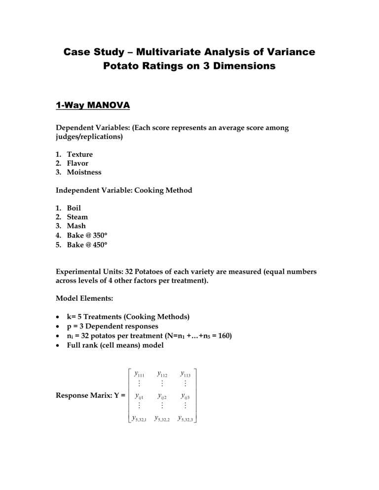
Full rank (cell means) model
 y111
 

Response Marix: Y =  yij1

 
 y5,32,1

y112

yij 2

y5,32, 2
y113 
 
yij3 

 
y5,32,3 
Here, Y represents a Nxp (160x3) matrix, where the first index (i) represents
treatment, the second (j) represents unit id withn treatment (replicate) and the
third index (k) represents the dependent response.
Measurements across units (potatos) are assumed independent, however the
dependent responses within a unit are not assumed independent. Let the
response vector for potato j within treatment i be labelled yij, then (Note that Y is
the vertical concatenation of the transpose of all yij vectors):
 y ij1 
yij =  y ij 2  with mean vector E(yij) =
 y ij3 
 
  i1 
   and Variance-covariance matrix
 i2 
  i 3 
 11  12  13 
V(yij)= =  21  22  23  which is symmetric.


 31  32  33 
The model matrix (X) and the parameter matrix () are (for the full rank model):
1
0

X= 0

0
0
0 0 0 0
1 0 0 0
0 1 0 0

0 0 1 0
0 0 0 1
and
 11

 21
 =   31

  41
  51
12
 22
 32
 42
 52
13 
 23 
 33 

 43 
 53 
where each element of the X matrix is a nix1 (32x1) column vector. That is, X is a
160x5 (Nxk) matrix. The model is of the form:
Y = X + 
Estimating  :
B = (X’X)-1X’Y =
  y1 j1
 j
0
0
0
0 
1 / 32
y 2 j1
 0
 
j
1
/
32
0
0
0


 0
0
1 / 32
0
0    y 3 j1

 j
0
0
0
1
/
32
0

   y 4 j1
 0
0
0
0
1 / 32  j
  y 5 j1
 j
y
y
y
y
y
1 j2
j
2 j2
j
3 j2
j
4 j2
j
5 j2
y
y
y
y
y
j


 y 11

2 j3


 y 21

3 j3
   y 31


 y 41
4 j3 
y

 51
5 j3 

1 j3
j
j
j
j
j
y 12
y 2 2
y 32
y 4 2
y 52
y 13 

y 2 3 
y 33 

y 4 3 
y 53 
where y i j is the sample mean for the jth dependent response for the ith treatment
group.
Estimating  :
= E[(yij - ij)( yij - ij)’]
 y i1 


From above, our estimate of ij is  y i2  so that an unbiased estimate of  is:
y 
 i 3 
  yij1   y i1  

1 k ni    

 yij1
S=
y

y
 ij 2
i 2 
N  k i 1 j 1    

  yij3  y i3  




yij 2
 
yij3  y i 1
y i 2
y i3

This can be computed in matrix form as:
S = (Y-XB)’((Y-XB)/(N-k) = Y’[I-X(X’X)-1X’]Y/(N-k)
Testing Equality of Mean Vectors Across Treatments
  i1 
Let i =   i 2  i=1,2,3,4,5. The vector is of length p in general, and there will be
  i 3 
k vectors.
We wish to test wheter the mean response vectors (Texture, Flavor, and
Moistness) are equal among cooking methods. That is:
H0: 1 = vs
HA: Not all i are equal
This test is of the form: Cfor:
1
0
C= 
0

0
0 0 0  1
1 0 0  1
and M = I5
0 1 0  1

0 0 1  1
Under H0, the model matrix X0 is a Nx1 column vector of 1’s and the parameter
matrix  is a row vector of the form  = 1  2  3  . The least squares
estimate of  is then:
B0=(X0’X0)-1X0’Y =
1  k ni
 Yij1
N  i 1 j 1
k
ni
k
Yij2
ni
Y
i 1 j 1
i 1 j 1
ij 3


  Y 1 Y 2

Y 3

Under H0, the matrix of the sums of squared errors and crossproducts can be
obtained as follows:
T = (Y-XB0)’(Y-XB0) =

( y ij1  y 1 ) 2


i
j

 ( y ij 2  y 2 )( y ij1  y 1 )
 i j

( y ij 3  y 3 )( y ij1  y 1 )
 
i
j
 ( y  y
 ( y
 ( y  y
ij1
i
1
j
ij 2
i
j
 y 2 )
2
j
ij 3
i
)( y ij 2  y 2 )
3
)( y ij 2  y 2 )

)( y ij 3  y 3 ) 


)(
y

y
)
ij 3
2
3

2


y
)
ij 3
3

 ( y  y
 ( y  y
 ( y
ij1
i
j
i
j
ij 2
i
j
1
Note that this is a multivariate version of the (corrected) total sum of squares.
Under HA the matrix of the sums of squared errors and crossproducts is
computed as follows:
E = (Y-XB)’(Y-XB) =

( y ij1  y i 1 ) 2


i
j

 ( y ij 2  y i 2 )( y ij1  y i 1 )
 i j

( y ij 3  y i 3 )( y ij1  y i 1 )
 
i
j
 ( y  y
 ( y
 ( y  y
ij1
i
i 1
j
ij 2
i
 y i2 )
2
i 3
)( y ij 2  y i  2 )

)( y ij 3  y i 3 ) 


)(
y

y
)
ij 3
i2
i 3

2

ij 3  y i 3 )

 ( y  y
 ( y  y
 ( y
ij1
i
j
i
j
ij 2
j
ij 3
i
)( y ij 2  y i  2 )
j
i
j
i 1
The between groups matrix of sums of squares and crossproducts is the
differeence between the matrices obtained under H0 and HA.
H=T–E=


2

i ni y i1  y 1


 ni y i2  y 2 y i1  y 1
 i
 n y y
i
i 3
3 y i 1  y 1
 
i




Test Statistics
Wilks’ Lambda:
 n y
i

 y 1 y i2  y 2
i 1

 n y  y 
  n y  y y  y
i
i2
2
i
i
i
i 3
3
i2
i
i 1
1
i 3
3
i
i2
2
i 3
3
i
2
i
  n y  y y  y 





n
y

y
y

y




 n y  y 

i
2
2
i
i
i 3
3

=det(E)/det(H+E) =
1
1 
where are the ordered eigenvalues of E-1H
i
this can be transformed to an approximate F-statistic:
1    rt  2u
1/ t
FW =
1 / t
with degrees of freedom: pq and rt-2u where:
pq
p = Number of dependent variables (3 in this example)
k = Number of treatments (groups) (5 in this example)
q = rank(C(X’X)-1C’) = k-1
r = (N-k) – (p-(k-1)+1)/2
u = (pq-2)/4
t=
p q
2
2

 4 / p2  q2  5
Pillai’s Trace
V = trace(H(H+E)-1) =

if p2+q2-5 > 0
(t = 1, otherwise)
i
1 
i
this can be transformed to an approximate F-statistic:
 2n  s  1  V 
FP = 

 with degrees of freedom s(2m+s+1) and s(2n+s+1) where:
 2m  s  1  s  V 
n = (N-k-p-1)/2
m = (|p-q|-1)/2
s = min(p,q)
Hotelling-Lawley Trace
U = trace(E-1H) =  i
this can be transformed to an approximate F-statistic:
FHL =
2( sn  1)U
with degrees of freedom: s(2m+s+1) and 2(sn+1)
s (2m  s  1)
2
Roy’s Largest Root
1
this can be transformed to an approximate upper bound for the F-statistic:
FR =
( N  k  r  q )
with degrees of freedom: r and N-k-r+q
r
SPSS output
r = max(p,q)
Descriptive Statistics
TEXTURE
FLAVOR
MOIST
COOKING
1
2
3
4
5
Total
1
2
3
4
5
Total
1
2
3
4
5
Total
Mean
2.4000
2.6031
2.5844
2.6563
2.4656
2.5419
2.9375
2.8063
2.9688
3.0375
2.8063
2.9113
2.2406
2.4156
2.6188
2.5063
2.3250
2.4213
Std. Deviation
.49774
.49350
.55014
.47311
.50648
.50736
.29044
.27349
.22781
.24854
.30684
.28284
.45851
.40965
.43138
.35372
.37845
.42432
N
32
32
32
32
32
160
32
32
32
32
32
160
32
32
32
32
32
160
Be twe en-Subj ects SSCP Matrix
Hy pothesis
Int ercept
COOKING
Error
TEXTURE
FLAVOR
MOIST
TEXTURE
FLAVOR
MOIST
TEXTURE
FLAVOR
MOIST
TEXTURE
1033.781
1184.005
984.722
1.427
.472
1.624
39.503
3.983
26.154
FLAVOR
1184.005
1356.060
1127.818
.472
1.343
.897
3.983
11.376
2.874
MOIST
984.722
1127.818
937.992
1.624
.897
2.821
26.154
2.874
25.807
Based on Type III Sum of Squares
1.427 0.472 1.624 


Note: H = 0.472 1.343 0.897


1.624 0.897 2.821
39.503 3.983 26.154
and E =  3.983 11.376 2.874 
26.154 2.874 25.807
Computations used to obtain elements of H:
H=
2

i ni y i1  y 1


 ni y i2  y 2 y i1  y 1
 i
 n y y
i
i 3
3 y i 1  y 1
 
i



Cooking method n



 n y
i

 y 1 y i2  y 2
i 1

 n y  y 
  n y  y y  y
i
i2
2
i
i 3
i
3
i2
i 1
1
i 3
3
i
i2
2
i 3
3
i
2
2
i
texture flavor
i
i
2
i
  n y  y y  y 





n
y

y
y

y




 n y  y 

i
i 3
3

i
moist
t*t (H11)
t*f (H12)
t*m (H13)
f*f (H22)
f*m (H23)
m*m (H33)
Boil
32 2.4000 2.9375
2.2406 0.64433952
-0.11896896
0.82052256
Steam
32 2.6031 2.8063
2.4156 0.11985408
-0.205632
-0.01116288
0.3528
Mash
32 2.5844 2.9688
2.6188
0.0578
0.0782
0.2686
0.1058
0.3634 1.2482
Bake @ 350
32 2.6563 3.0375
2.5063 0.41879552
0.46199296
0.311168
0.5096461
0.343264 0.2312
2.325 0.18629408
0.256368
0.23512608
0.47196
1.62425376
Bake @ 450
Overall
32 2.4656 2.8063
160 2.5419 2.9113
2.4213
1.4270832
0.0219661 -0.15149888 1.04487968
0.3528
E=
 ( y  y
 ( y
 ( y  y
ij1
i
i 1
j
ij 2
i
 y i2 ) 2
j
ij 3
i
)( y ij 2  y i  2 )
j
i 3
)( y ij 2  y i  2 )

)( y ij 3  y i 3 ) 


)(
y

y
)
ij 3
i2
i 3

2


y
)
ij 3
i 3

 ( y  y
 ( y  y
 ( y
ij1
i
j
i
j
ij 2
i
j
i 1
Too many calculations to write out (each element based on 160 terms).
The Test Statistics are obtained below:
0.323568 0.29675808
1.3430122 0.89788512 2.82207744
Computations used to obtain E:

( y ij1  y i 1 ) 2


i
j

 ( y ij 2  y i 2 )( y ij1  y i 1 )
 i j

( y ij 3  y i 3 )( y ij1  y i 1 )
 
i
j
0.019152 0.00103968
Multivaria te Testsc
Effect
Int ercept
COOKING
Pillai's Trac e
W ilks' Lambda
Hotelling's Trac e
Roy's Largest Root
Pillai's Trac e
W ilks' Lambda
Hotelling's Trac e
Roy's Largest Root
Value
.993
.007
137.677
137.677
.263
.755
.301
.196
F
Hy pothesis df
7021.522a
3.000
a
7021.522
3.000
7021.522a
3.000
7021.522a
3.000
3.719
12.000
3.783
12.000
3.809
12.000
7.591b
4.000
Error df
153.000
153.000
153.000
153.000
465.000
405.091
455.000
155.000
Sig.
.000
.000
.000
.000
.000
.000
.000
.000
a. Ex act stat istic
b. The st atist ic is an upper bound on F that yields a lower bound on the significance level.
c. Design: Int ercept+COOKING
Matrix Computations to obtain the test statistics (SAS/IML):
Wilks’ Lambda
det(E) = 3678.767
det(E+H) = 4872.5205
3678.767/4872.5205 = 0.7550
p = Number of dependent variables = 3
k = Number of treatments (groups) = 5
q = rank(C(X’X)-1C’) = k-1 = 4
r = (N-k) – (p-(k-1)+1)/2 = (160-5)- (3-(5-1)+1)/2 = 155-0 = 155
u = (pq-2)/4 = (3(4)-2)/4 = 2.5
t=
p q
2
2


 4 / p 2  q 2  5  ((9)(16)  4) /(9  16  5)  140 / 20  7  2.646
FW =
1  1 / t rt  2u (1  0.7551 / 2.646 ) 155(2.646)  2(2.5) (0.1008)( 405.13) 40.837



 3.785
pq
3(4)
(0.8992)(12)
10.790
1 / t
0.7551 / 2.646


with degrees of freedom: pq=3(4)=12 and rt-2u = 405.13
Pillai’s Trace
H(H+E)-1 =
-0.011883 0.0218476 0.065365
-0.034392 0.102481 0.051215
-0.082422 0.0483715 0.1721382
V = trace(H(H+E)-1) = -0.011883+0.102481+0.1721382 = 0.2627
n = (N-k-p-1)/2 = (160-5-3-1)/2 = 151/2 = 75.5
m = (|p-q|-1)/2 = (|3-4|-1)/2 = 0
s = min(p,q) = min(3,4) = 3
FP =
 2n  s  1  V   2(75.5)  3  1  0.2627  (155)(0.2627) 40.72


 3.72


  

(4)( 2.7373)
10.95
 2m  s  1  s  V   2(0)  3  1  3  0.2627 
df: s(2m+s+1) = 3(2(0)+3+1) = 12 and s(2n+s+1) = 3(2(75.5)+3+1) = 465
Hotelling-Lawley Trace
E-1H =
-0.01915 -0.043302 -0.100184
0.0281437 0.1166674 0.0624443
0.0791854 0.0656628 0.203884
U = trace(E-1H) = -0.01915 + 0.1166674 + 0.203884 = 0.3014
FHL =
2( sn  1)U
2(3(75.5)  1)(0.3014) 137.137


 3.809
36
s (2m  s  1)
3 2 (2(0)  3  1)
2
df: s(2m+s+1) = 3(2(0)+3+1) = 12 and 2(sn+1) = 2(3(75.5)+1) = 455
Roy’s Largest Root
Eigenvalues of E-1H:
1 = 0.1959 2 = 0.0802 3 = 0.0253
1 = 0.1959
this can be transformed to an approximate upper bound for the F-statistic:
FR =
( N  k  r  q) 0.1959(160  5  4  4) 30.3645


 7.59
r
4
4
degrees of freedom: r = max(3,4) = 4 and N-k-r+q = 160-5-4+4 = 155
Testing Equality of Variance-Covariance Matrices Across Treatments
Estimated variance-covariance matrix for treatment i
Si = (Yi-(1/ni)JYi)’ (Yi-(1/ni)JYi)/(ni-1)
i=1,…,k
Where:
 Yi is a nixp matrix of dependent responses from treatment i
 J is a nixni matrix of 1’s
 (1/ni)JYi is a nixp matrix with each row containing the mean for each response with
each row being: y i1 y i2 y i3 in the current example (with ni=32)


H0: k (Common Covariance matrices across groups)
Testing Procedure:
Compute:
k
S=
 (n
i 1
i
 1) Si / (N-k) = E/(N-k)
k
W = (N-k)log(|S|)   (ni  1) log(|Si|)
i 1
C
2 p  3p 1  k 1
1 



6( p  1)( k  1)  i 1 ni  1 N  k 
f 
p ( p  1)( k  1)
2
2
When ni > 20 and p and k are less than 6 (which holds in our case):
X 2  (1  C )W ~  2 ( f ) (approximately)
F-approximation:
C0 
f0 
a

( p  1)( p  2)  k
1
1


2
2 
6(k  1)  i 1 ni  1
N  k  
f 2
C0  C 2
f
1  C  ( f / f0 )
b
f0
1  C  (2 / f 0 )
Case 1: C0 – C2 > 0
 F = W/a ~ F(f , f0)
(approximately)
Case 2: C0 – C2 < 0
 F = W/b ~ F(f , f0)
(approximately)
SPSS Results of Box’s Test:
Box's Test of Equality of Covariance Matrices a
Box's M
F
df1
df2
Sig.
27.200
1.085
24
66334.513
.351
Tests the null hypothesis that the obs erved covariance
matrices of the dependent variables are equal across groups.
a. Design: Intercept+COOKING
Matrix Computations (SAS/IML)
.2477 .0335 .1961
S1 = .0335 .0844 .0255
.1961 .0255 .2102 
.2435 .0222 .1774
S2 = .0222 .0748 .0134
.1774 .0134 .1678
 .3027  .0099 .1661 
S3 =  .0099 .0519  .0049 S4 =


 .1661  .0049 .1861 
.2238 .0494 .1458
.0494 .0618 .0310


.1458 .0310 .1251
.2565 .0331 .1583
S5 = .0331 .0942 .0276
.1583 .0276 .1432
I
n_I-1
1
2
3
4
5
overall
31
31
31
31
31
155
.2549 .0257 .1687 
S = .0257 .0734 .0185


.1687 .0185 .1665
|S_I|
log(|S_I|) (n-1)log(|S|)
0.001087 -6.82479 -211.56861
0.000683 -7.28931 -225.96857
0.001482
-6.5147 -201.95571
0.000343 -7.97661 -247.27505
0.001037 -6.87181 -213.02608
0.000988 -6.91993
-1072.589
W = -1072.59-(-211.57-225.97-201.96-247.28-213.03) = 27.21
SPSS)
(This is Box’s M in
2(3) 2  3(3)  1  k
1
1  26  24 


 0.041936


6(3  1)(5  1)  i 1 32  1 160  5  96 155 
3(3  1)(5  1) 48
f 

 24
2
2
C
C0 
f0 
a
 10  124 
(3  1)(3  2)  k
1
1


 0.0021505

2
2 
6(5  1)  i 1 32  1
160  5  24  1552 
24  2
0.0021505  (.041936) 2

26
 66348.2
.000392
24
24

1  0.041936  (24 / 66348.2) .9577
Case 1: C0 – C2 > 0
(approximately)
 25.06
 F = W/a = 27.21/25.06 =1.086 ~ F(24 , 66348)
Do not conclude that the population variance-covariance matrices differ among
cooking methods.
Bartlett’s Test for Sphericity (Independence among responses)
H0:  = 2I
Compute:
 = {|S| / [trace(S) / p]p}
f = (p-1)(p+2)/2
C = (2p2+p+2) / (6p(N-k))
X2 = -(N-k)(1-C)log() ~ 2(f)
(approximately)
SPSS results of Bartlett’s Test:
Bartlett's Test of Sphericity(a)
Likelihood Ratio
Approx. Chi-Square
df
.000
232.579
5
Sig.
.000
Tests the null hypothesis that the residual covariance matrix is proportional to an identity matrix.
a Design: Intercept+COOKING
Matrix Computations (SAS/IML)
|S| = 0.0009878
trace(S) = 0.2549 + 0.0734 + 0.1665 = 0.4948
= 0.0009878 / (.4948/3)3 = 0.220163
f = (2)(5)/2 = 5
C = (2(3)2 + 3 + 2) / (6(3)(160-5)) = 23 / 2790 = 0.008244
X2 = -(160-5)(1-0.008244)log(0.220163) = -155(0.991756)(-1.5134) = 232.64
Strong evidence that the variance-covariance matrix is not proportional to the
identity matrix.