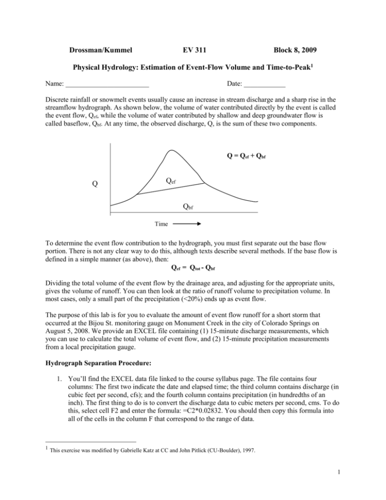
Drossman/Kummel
EV 311
Block 8, 2009
Physical Hydrology: Estimation of Event-Flow Volume and Time-to-Peak1
Name: ________________________
Date: ____________
Discrete rainfall or snowmelt events usually cause an increase in stream discharge and a sharp rise in the
streamflow hydrograph. As shown below, the volume of water contributed directly by the event is called
the event flow, Qef, while the volume of water contributed by shallow and deep groundwater flow is
called baseflow, Qbf. At any time, the observed discharge, Q, is the sum of these two components.
Q = Qef + Qbf
Q
Qef
Qbf
Time
To determine the event flow contribution to the hydrograph, you must first separate out the base flow
portion. There is not any clear way to do this, although texts describe several methods. If the base flow is
defined in a simple manner (as above), then:
Qef = Qtot - Qbf
Dividing the total volume of the event flow by the drainage area, and adjusting for the appropriate units,
gives the volume of runoff. You can then look at the ratio of runoff volume to precipitation volume. In
most cases, only a small part of the precipitation (<20%) ends up as event flow.
The purpose of this lab is for you to evaluate the amount of event flow runoff for a short storm that
occurred at the Bijou St. monitoring gauge on Monument Creek in the city of Colorado Springs on
August 5, 2008. We provide an EXCEL file containing (1) 15-minute discharge measurements, which
you can use to calculate the total volume of event flow, and (2) 15-minute precipitation measurements
from a local precipitation gauge.
Hydrograph Separation Procedure:
1. You’ll find the EXCEL data file linked to the course syllabus page. The file contains four
columns: The first two indicate the date and elapsed time; the third column contains discharge (in
cubic feet per second, cfs); and the fourth column contains precipitation (in hundredths of an
inch). The first thing to do is to convert the discharge data to cubic meters per second, cms. To do
this, select cell F2 and enter the formula: =C2*0.02832. You should then copy this formula into
all of the cells in the column F that correspond to the range of data.
1
This exercise was modified by Gabrielle Katz at CC and John Pitlick (CU-Boulder), 1997.
1
2. Make a scatter plot (connect lines without points option) of all the discharge data (a hydrograph)
for the three-day interval on a separate worksheet. Label the worksheet Hydro. How do the
hydrographs of storm events differ from each other? Why?
3. The next step involves numerically separating the event flow volume for the earliest storm event
from the base flow volume for the same event on your hydrograph. Re-scale the graph to plot the
storm flow from t=5.0 hr to t=12.5 hr. What are the respective discharge values for the beginning
and end values of flow during the storm (in cms)? Using the ‘line’ tool from the drawing toolbar,
draw a line connecting the beginning and the end of the event. (choose: View  Toolbars 
Drawing). Compare this to the drawing on the first page and discuss which area of the
hydrograph represents base flow and which area represents storm (event) flow.
4. The base flow contribution (though small) should be subtracted from each of the observations of
Q, but this is straightforward because we will assume that the base flow increases linearly
between t=7.25 and t=12.25 hr. To do this, we will use the EXCEL linear regression command.
The steps are as follows: (i) somewhere at the right hand side of the page, enter the values 7.25
and flow in two adjacent columns, and 12.25 and corresponding flows in adjacent rows in the
columns below as shown:
7.25
12.25
flow at 7.25 hrs
flow at 12.25 hrs
(ii) select one cell (beneath these cells) and calculate the line slope (m) with the following
formula: =SLOPE(cellsy, cellsx), where cellsy is the range of cells containing your y
values, and cellsx is the range of cells with your x values.
(iii) select another empty cell and calculate the line intercept (b), with this formula:
=INTERCEPT(cellsy, cellsx)
5. Using the line equation, Qbf = m t + b, compute the base flow for any time t during the storm
event. Find the cell in column F that corresponds to t=7.5 and enter a formula in column G
corresponding to this equation by typing in your values for m and b in the formula. This is Qbf.
6. In the next column (H), type in a formula to calculate the event flow for each time, by subtracting
the base flow from the observed Q. This is Qfc.
7. Next, we can numerically integrate the area under the hydrograph and determine the total amount
of event flow volume. The average volume of flow contributed in each time period (tn to tn+1) is
the product of the average flow and the time interval (900 seconds = 15 minutes):
Qn 1  Qn 

* t n 1  t n * 900sec
 2

Enter a formula corresponding to this equation in the appropriate row in column I and do a fill down
to t=12.25 hr. At the bottom of this column, calculate the total event flow volume by summing the
range of computed 15-minute
event flow volumes.

Total volume of event flow: __________ m3
2
8. Next, we can compare the amount of runoff to the amount of precipitation. At this point, the total
runoff is expressed as a volume, while precipitation is expressed as a depth. To convert the
precipitation depth (m) to volume (m3), you must multiply by the drainage area, which must first
be converted to the same units (miles2 * 2.590 = km2, and km2 = 1,000,000 m2).
Drainage area (at Bijou gauge #07104905) = 235 miles2 = __________ km2 = ___________ m2
Depth of precipitation event on 08/05/08 = 0.11 inches = _________ cm = ____________ m
Precipitation volume (m3) = Watershed area (m2) * Precipitation depth (m) = __________ m3
Questions to consider:
 What is the ratio of the volume of runoff to the volume of precipitation for this event?
 What percent of the precipitation made it to Monument Creek?
 Can you think of some reasons why significantly less than 100% makes it to the creek?
 Where else did/could the water go?
 Hypothesize why the subsequent storm events look wider than this first event?
Time to Peak Procedure.
1. First, convert the precipitation values from inches (in D) to cm (in E) (1 inch = 2.54 cm).
2. To add the precipitation values to your graph, select the chart and then go to Chart  add Data,
and select the range of cells containing the precipitation data. The data series should appear on
the chart, but not relative to the correct scale. To fix this, double click on the precipitation data
points on the graph, and then in the pop-up-window, choose: Axis  Secondary axis. This will
relate the precipitation data to their own y-axis values.
3. Look at the difference in timing between the observed peak discharge, Qpk, and the measured
maximum precipitation. This time period, called time to peak (tpk) reflects many physical
parameters (e.g. characteristics of the precipitation event, climate, and physical drainage basin
characteristics). It may also reflect data collection characteristics (e.g. relative locations of the
stream gauge and the precipitation gauge).
Questions to ponder:
 What is the observed time to peak?
 Does this appear to change for later peaks?
 What physical attributes of our drainage basin and our local climate likely account for the
observed pattern?
 Relate your observation to the STELLA hydrograph model in the next exercise.
Make sure you understand how to use Excel and the data analysis methods as they will be useful for
the weekend hydrology project.
3