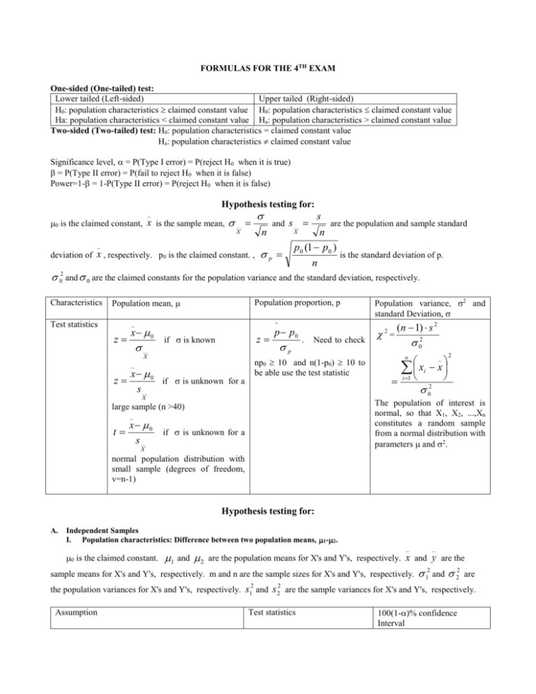
FORMULAS FOR THE 4TH EXAM
One-sided (One-tailed) test:
Lower tailed (Left-sided)
Upper tailed (Right-sided)
H0: population characteristics  claimed constant value H0: population characteristics  claimed constant value
Ha: population characteristics < claimed constant value Ha: population characteristics > claimed constant value
Two-sided (Two-tailed) test: H0: population characteristics = claimed constant value
Ha: population characteristics  claimed constant value
Significance level,  = P(Type I error) = P(reject H0 when it is true)
 = P(Type II error) = P(fail to reject H0 when it is false)
Power=1- = 1-P(Type II error) = P(reject H0 when it is false)
Hypothesis testing for:
_
0 is the claimed constant, x is the sample mean,

 
__
and
n
X
_
deviation of x , respectively. p0 is the claimed constant. ,
s
s __ 
are the population and sample standard
n
p0 (1  p0 )
is the standard deviation of p.
n
X
p 
 02 and  0 are the claimed constants for the population variance and the standard deviation, respectively.
Characteristics
Population mean, 
Test statistics
Population proportion, p
_
z
x  0

^
z
if  is known
__
X
p
.
Need to check
np0  10 and n(1-p0)  10 to
be able use the test statistic
_
z
p  p0
x  0
if  is unknown for a
s __
Population variance, 2 and
standard Deviation, 
2=
(n  1)  s 2
 02
_


x

x



i

i 1 

2
n
2
0
X
The population of interest is
normal, so that X1, X2, ...,Xn
constitutes a random sample
from a normal distribution with
parameters  and 2.
large sample (n >40)
_
x  0
t
if  is unknown for a
s __
X
normal population distribution with
small sample (degrees of freedom,
v=n-1)
Hypothesis testing for:
A.
Independent Samples
I. Population characteristics: Difference between two population means, 1-2.
0 is the claimed constant.
1 and  2
_
sample means for X's and Y's, respectively. m and n are the sample sizes for X's and Y's, respectively.
the population variances for X's and Y's, respectively.
Assumption
_
are the population means for X's and Y's, respectively. x and
2
1
y are the
 12 and  22
2
2
are
s and s are the sample variances for X's and Y's, respectively.
Test statistics
100(1-)% confidence
Interval
both popn. distributions are normal and
are known
 12 ,  22
_ _
 x y    0

z
 12
m
large sample size (m>40 and n>40) and
are unknown
 ,
2
1
2
2
sample size is small where unknown
 12 ,  22
are
assumed to be different (  1   2 ) and degrees of
2
2
2
 s12 s 22 
  
m n
freedom, v 
2
2
s12 / m
s2 / n
 2
m 1
n 1

 
n
s12 s 22
_ _
x

y

z


  /2
m n


_ _
 x y    0

,
t
1 1
sp

m n
(m  1) s12  (n  1) s 22
s 2p 
mn2
1 1
_ _

 x  y   t / 2 ;v s p
m n


_
s2 s2
_ _
 x  y   t / 2 ; v 1  2
m n



both popn. distributions are normal and at least one
sample size is small where unknown
 ,
2
1
2
2
are
assumed to be the same (  =  ) and degrees of
2
1
2
2
freedom, v  m  n  2 is used to look up the
critical values.
II.
 22


 x y    0

z
2
s1 s 22

m n
_ _
 x y    0

t
2
s1 s 22

m n
_
both popn. distributions are normal and at least one

 12  22
_ _

 x  y   z / 2
m
n


Population characteristics: Difference between two population proportions, p1-p2.
^
^
p0 is the claimed constant. p 1 and p 2 are the sample proportions for X's and Y's, respectively.
p1 and p 2 are the
population proportions for X's and Y's, respectively. m and n are the large sample sizes for X's and Y's, respectively. The
^
estimator for p is p 
Test statistics:
z
X Y
m ^
n ^

p1 
p2
mn mn
mn
^
^

 p1  p 2   p0


,
^
^
1
1




p1  p   

 m n 


^
^


100(1-)% large sample confidence Interval:  p1  p 2   z / 2
^
^
^
^




p1 1  p1  p 2 1  p 2 

 

m
n
 12 /  22 or standard deviations,  1 /  2 .
 12 and  22 are the population variances for X's and Y's,
III. Population characteristics: Ratio of the two population variances,
X and Y's are random sample from a normal distribution.
2
respectively. s1 and
Y's, respectively.
s 22 are the sample variances for X's and Y's, respectively. m and n are the sample sizes for X's and
s12 / s 22
 12
s12 / s 22
s12
2
2


Test statistics: F  2 . 100(1-)% confidence Interval for  1 /  2 :
F / 2;m 1,n 1  22 F1 / 2;m 1,n 1
s2
B.
Dependent Samples- Paired Data
Population characteristics: Difference between two population means, D =1-2.
0 is the claimed constant. Assumption: the difference distribution should be normal.
_
Test statistics: t 
d  0
sD / n
_
where D=X-Y and d and
s D are the corresponding sample average and the standard
deviation of D. Both X and Y must have n observations. The degrees of freedom to look at the table is v=n-1
_
sD
100(1-)% confidence Intervals with the same assumptions: d  t / 2;n 1
n
Decision can be made in one of the two ways in Parts I, II, and III for single population characteristics or the comparing
two poulations:
a. Let z* or t* be the computed test statistic values.
if test statistics is z if test statistics is t
Lower tailed test P-value = P(z<z*)
P-value = P(t<t*)
Upper tailed test P-value = P(z>z*)
P-value = P(t>t*)
Two-tailed test
P-value = 2P(z>|z*|) P-value = 2P(t > |t*| )
In each case, you can reject H0 if P-value   and fail to reject H0 (accept H0) if P-value > 
b.
Rejection region for level  test:
test statistics is z
test statistics is t
test statistics is
2
test statistics is F
Lower tailed test
z  -z
t  -t;v
 2 <  12 ;n1
F  F1-;m-1,n-1
Upper tailed test
z  z
t  t;v
 2 >  2;n1
F  F;m-1,n-1
Two- tailed test
z  -z/2 or z  z/2
t  -t/2;v or t  t/2;v
 2 <  12 / 2;n1 or  2 >  2 / 2;n1
F  F1-/2;m-1,n-1 or
F  F/2;m-1,n-1
Do not forget that, F1-/2;m-1,n-1 = 1 / F/2;n-1,m-1 for the F-table
Single Factor ANOVA :
Model:
X ij   i   ij
treatment).
X ij : observations ,
or
X ij     i   ij
 i : ith treatment mean,
where i=1,...,I (number of treatments), j=1,...,J (number of observations in each
 i   i   : ith treatment effect.
 ij : errors which are normally distributed with mean, 0 and the constant variance,  2 .
Assumptions:
X ij 's are independent (  ij 's are independent).  ij 's are normally distributed with mean, 0 and the constant variance,
 2 . X ij 's are normally distributed with mean,  i
Hypothesis:
Or
H 0 : 1  ...   I 1   I
H0 :i  0
for all i versus
versus
and the constant variance,
2.
H a : at least one  i   j
for
i j
where
 i .and  j 's are treatment means.
H a :  i  0 for at least one i where  i is the ith treatment effect.
Analysis of Variance Table:
Source
df
SS
MS
F
Prob > F
Treatments
I-1
SSTr
MSTr = SStr / (I-1)
MSTr / MSE
P-value
Error
I(J-1)
SSE
MSE = SSE / [I(J-1)]
Total
IJ-1
SSTotal
where df is the degrees of freedom, SS is the sum of squares, MS is the mean square. Reject H 0 if the P-value  or if the test statistics
F > F;I-1,I(J-1). If you reject the null hypothesis, you need to use multiple comparison test such as Tukey-Kramer
I
For the case of unequal sample sizes, let
n   Ji
and j=1,…,Ji . Then the difference in the analysis of variance table and multiple
i 1
comparison test is as follows.
Source
Treatments
Error
Total
Df
I-1
n-I
n-1
SS
SSTr
SSE
SSTotal
MS
MSTr = SStr / (I-1)
MSE = SSE / (n-I)
F
MSTr / MSE
Prob > F
P-value
where df is the degrees of freedom, SS is the sum of squares, MS is the mean square. Reject H 0 if the P-value or if the test statistics
F > F;I-1,n-I. If you reject the null hypothesis, you need to use multiple comparison test such as Tukey-Kramer to see which means are
different.
Confidence Interval for
   ci  i
:
c
MSE  ci2
_
i
x i  t / 2; I ( J 1)
J
i
i
Simple Linear Regression and Correlation
PEARSON’S CORRELATION COEFFICIENT :measures
the strength & direction of the linear relationship between X and Y. X
and Y must be numerical variables,
r
 X
i
 X Yi  Y 
(n  1) s x s y
 X  X Y  Y 
 X  X   Y  Y 

i
i
2
2
i
i
where sx and sy are the standard deviations for x and y. Notice we are looking at how far each point deviates from the average X and Y
value.
H 0 :  XY  0
(the true correlation is zero) versus
The formal test for the correlation has the test statistics
H a :  XY  0
t
r n2
1 r2
(the true correlation is not zero).
with n-2 degrees of freedom.
Minitab gives you the following output for simple linear regression:
parameters
0
and
Predictor (y)
Y   0  1 x  e ,
where n observations included, the
 1 are constants whose "true" values are unknown and must be estimated from the data.
Coef
SE Coef
T
Constant
b0
sb0
b0
s b0
p-value for
Ha : 0  0
Independent(x)
b1
s b1
b1
s b1
p-value for
H a : 1  0
Analysis of Variance
Source
DF
Regression
Residual Error
Total
SS
P
MS
F
1
SSR
MSR=SSR/1
MSR/MSE
n-2
n-1
SSE
SST
MSE=SSE/(n-2)
P
p-value for
H a : 1  0
Coefficient of Determination, R2 : Measure what percent of Y's variation is explained by the X variables via the regression model. It
tells us the proportion of SST that is explained by the fitted equation. Note that SSE is the proportion of SST that is not explained by the
model.
SSR
SSE
 1
.
SST
SST
H 0 : 1  10
R2 
Only in simple linear regression,
R 2  r 2 where r is the Pearson’s correlation coefficient.
H a : 1  10
Test statistics:
t
b1   10
s b1
where
 10 is the value slope is compared with.
Decision making can be done by using error degrees of freedom for any other t test we have discussed before (either using the P-value or
the rejection region method).
The 100(1-)% confidence interval for
 1 is b1  t / 2;df sb
1