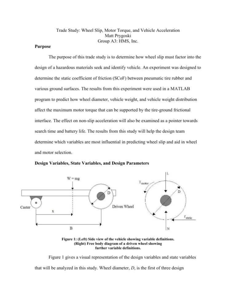
Trade Study: Wheel Slip, Motor Torque, and Vehicle Acceleration
Matt Prygoski
Group A3: HMS, Inc.
Purpose
The purpose of this trade study is to determine how wheel slip must factor into the
design of a hazardous materials seek and identify vehicle. An experiment was designed to
determine the static coefficient of friction (SCoF) between pneumatic tire rubber and
various ground surfaces. The results from this experiment were used in a MATLAB
program to predict how wheel diameter, vehicle weight, and vehicle weight distribution
affect the maximum motor torque that can be supported by the tire-ground frictional
interface. The effect on non-slip acceleration will also be examined as a pointer towards
search time and battery life. The results from this study will help the design team
determine which variables are most influential in predicting wheel slip and aid in wheel
and motor selection.
Design Variables, State Variables, and Design Parameters
Figure 1: (Left) Side view of the vehicle showing variable definitions.
(Right) Free body diagram of a driven wheel showing
further variable definitions.
Figure 1 gives a visual representation of the design variables and state variables
that will be analyzed in this study. Wheel diameter, D, is the first of three design
variables analyzed. D varies from 10 cm to 30 cm, which reflects the range of
commercially available pneumatic wheels. The second design variable, x, reflects the
position of the center of gravity (CoG) along the midline of the vehicle. To avoid tipping,
x must lie between the wheels and casters with an estimated 10 cm buffer on either side.
Since the wheelbase, B, of the vehicle is 60 cm, x ranges from 10 cm to 50 cm. The third
design variable is the mass, m, of the vehicle which ranges from 10 kg to 30 kg. It is
unlikely a vehicle would be less than 10 kg due to the lack of lightweight components,
and weighing above 30 kg would overstress the motors and battery. While x and m may
usually be considered state variables, they are taken to be design variables in this study.
Adding ballast (like sandbags in a pickup truck) can change m, and changing the position
of heavy components, like the batteries, changes x.
State variables include the load, L, supported by one wheel, the normal force, N,
and the frictional force, fstatic, that can be supplied by the ground. One state variable that
will be used to judge merit is the maximum motor torque, Tmotor-max, that can be supported
by the frictional interface. Tmotor-max must be between .1 Nm and 5 Nm to be applicable to
the motors we will likely use. A higher value of Tmotor-max is better because this means
more torque can be transmitted without slip. The second state variable used to judge
merit is a, or the acceleration of the vehicle, and must not exceed 9.81 m/s2 to avoid
breaking components. Values will likely be much lower, and are an indication of search
time and battery life. Higher values of a, for a given non-slip motor torque, are preferred.
The most important design parameter is the SCoF, or μs. The value of μs depends
on the surface the vehicle is traveling on. It should be independent of the vehicle weight
and surface area of the interface. An experiment was designed and performed to
determine the value of μs for different surfaces assuming a Coulomb friction model. The
experimental results proved this to be a valid assumption. For this trade study a value of
μs = .70 was adopted. This was the lowest average value that a surface (dirt) had, and was
conservatively chosen to limit the chance of wheel slip. More information on the
experiment and the experimental results can be found in Appendix 1.
Mathematical Model
A mathematical model was developed from the free body diagram presented in
Figure 1. In this diagram, L is the load carried by one wheel, calculated from a moment
summation about the casters. This is counteracted by the normal force, N, supplied by the
ground. The wheel is turned by a motor torque, Tmotor. For the wheel to turn without
slipping, the motor torque must be less than the maximum torque that can be supplied by
friction with the ground. For this vehicle, the frictional resistive force that can be supplied
by the ground is
f static   staticN   staticL 
 staticWx
2B
[1]
This force acts with a moment arm equal to the radius of the wheel, so the torque that can
be supplied by friction is
T friction 
 staticND
2

 staticLD
2

 staticWxD
4B
[2]
At the verge of slip, Tmotor-max equals Tfriction. When Tmotor is well below Tmotor-max, the
acceleration of the car is calculated to be
a 
4T
Dm
[3]
A MATLAB program was written to calculate the changes in Tmotor-max and a
while varying one design variable at a time from its minimum to maximum value. The
design variables were held at their average value if their effect was not being isolated.
As mentioned before, this analysis is based on a Coulomb friction model which is
probably not accurate for surfaces like grass and dirt. Many other factors like surface
indentation, tire pressure, tire tread, and the self-lubricating nature of broken grass blades
are relevant but not addressed. But, based on the experimental results, this model should
give a good approximation of sliding/slipping. This model also ignores dynamic forces,
inclined surfaces, and side-to-side weight imbalances on the vehicle. These issues would
be important to consider in a more advanced model.
Mathematical Results
Figures 2 and 3 are provided to show how Tmotor-max and a are affected as each
design variable is varied. To aid in comparison, the values of the design were normalized
with respect to percentage of total range. For instance 0% corresponds to a wheel
diameter of 10 cm and 100% corresponds to D = 30 cm.
Figure 2 shows that the value of x has the largest influence on Tmotor-max, followed
by D, and then m. This is useful because x can be manipulated simply through vehicle
layout which may be very flexible. Also, adding weight may beget other problems, so it
is good to know it has the smallest effect on wheel slip.
Figure 2: Maximum Torque before wheel slip. Each design variable varied from 0-100% while others
held at 50% of their range
Figure 3: Vehicle acceleration at an arbitrary input torque of 2 Nm (assuming no slip). Each design
variable varied from 0-100% while others held at 50% of their range
Figure 3 shows that x has no bearing on normal vehicle acceleration so it can be changed
without consequence. Increasing D and m decrease a, even though they serve to increase
traction. This is a trade off that must be examined further.
Figure 4: Torque before wheel slip for select vehicle weights as wheel diameter is varied. The limit of
5 Nm on the state variable is reflected in this graph.
The analysis indicates that x should be maximized at 50 cm. At this value of x, Figure 4
shows how mass and wheel diameter affect Tmotor-max. Combinations of D and m that yield
a Tmotor-max above 5 Nm are unnecessary since 5 Nm is a constraint on the motor torque,
however being above this threshold this will ensure that slip does not occur.
Influence on Design
The results from this trade study give insight into how to control wheel slip. First,
the position of the CoG of the vehicle should be placed as close to the rear wheels as
possible (x = 50 cm). It is the most influential in determining torque before slip, and has
no adverse effects on acceleration. It can also be tuned purely through design of the
vehicle layout, rather than component selection. Vehicle mass is the least influential on
maximum motor torque and acceleration. It would be advisable to treat mass more like a
state variable, resulting from other design choices, and only add ballast to the vehicle as a
last resort. This would simplify the design space and prevent problems associated with
adding otherwise useless weight to the vehicle. Wheel diameter is then the last variable
that must be chosen. Estimating the vehicle weight, Figure 4 can be used to pick a wheel
diameter for a motor with a given torque rating. Or, a motor can be sized for a specific
wheel diameter if the weight is known. Either way, the wheel should be as small as
possible without risking slip so that it does not hinder vehicle acceleration (as shown in
Figure 3). It is important to note that the numbers presented in the plots were derived
from an experimentally determined SCoF. The MATLAB program can regenerate the
plots if a different value of μs is applicable. This trade study has independently shown
how various factors affect wheel slip and has also provided experimental friction data for
different surfaces. When used in conjunction with another trade study on motor power,
the design team should have a clear picture of how to size the motors and wheels based
on the vehicle weight and vehicle weight distribution.
Appendix
1) Experimental Analysis and Results
2) Rough Experimental Data
3) MATLAB Mathematical Model Code
Appendix 1
Experimental Analysis and Results
Figure A: Experimental setup. Clockwise from top left: weighing the sled; pull test on wet grass;
moist grass; dirt; sidewalk; rubber gym flooring
An experiment was designed to determine μs for five different surfaces. A friction
test sled was constructed for use in the experiment, which is shown in Figure A. The sled
has sections of a pneumatic tire mounted on the undersides of its runners. It has a post
located in the center of the sled to rack weights on. It also has a hook on the front for
attachment to a spring scale. The spring scale determines the total weight of the vehicle
as well as the force needed to accelerate the sled from a standstill. The ratio of the pull
force to the weight is defines μs.
Five surfaces were tested. Wet grass, dry grass, dirt, and concrete were examined
because they could be encountered by the vehicle. A rubber gym flooring was also tested
as a control. For each surface, the sled was tested at a weight of 7.5 kg, 12.0 kg, 16.5 kg,
and 21.0 kg, with three runs at each weight. The SCoF proved to be fairly independent of
the sled weight, which is in line with friction theory. Data is more scattered on the grass
surfaces due to surface irregularity.
Figure B: Static Coefficient of Friction values for different surfaces with varying normal force. Note
that the first four bars of each surface’s data are the average of three tests.
Figure B provides a summary of the average SCoF values for each load and surface. The
highest SCoF, for concrete, would provide an upper limit for sizing motors. This study
will adopt a value of μs = .70, or the average value seen for dirt. This is the lowest
average value seen for any surface and was chosen as a conservative estimate to limit the
chances of wheel slip.
Appendix 2
Rough Friction Data
Surface
Vehicle Mass (kg) Test # Pull Load (kg)
Grass
Grass
Grass
Grass
Grass
Grass
Grass
Grass
Grass
Grass
Grass
Grass
1
1
1
1
1
1
1
1
1
1
1
1
Low
Low
Low
Med-Low
Med-Low
Med-Low
Med-High
Med-High
Med-High
High
High
High
1
2
3
1
2
3
1
2
3
1
2
3
7.5
4.5
5.5
8.5
9.5
9
13
13
13.5
17
14.5
14
1
0.6
0.73
0.71
0.79
0.75
0.79
0.79
0.81
0.81
0.69
0.66
Grass
Grass
Grass
Grass
Grass
Grass
Grass
Grass
Grass
Grass
Grass
Grass
2
2
2
2
2
2
2
2
2
2
2
2
Low
Low
Low
Med-Low
Med-Low
Med-Low
Med-High
Med-High
Med-High
High
High
High
1
2
3
1
2
3
1
2
3
1
2
3
7
6.5
7
11
11.5
10.5
15
15
16
19
18
19
0.93
0.87
0.93
0.92
0.96
0.88
0.91
0.91
0.97
0.9
0.86
0.9
Low
Low
Low
Med-Low
Med-Low
Med-Low
Med-High
Med-High
Med-High
High
High
High
1
2
3
1
2
3
1
2
3
1
2
3
5
5.5
5
9.5
8
8.5
13
11
11.5
14.5
15.5
14
0.67
0.73
0.67
0.79
0.67
0.71
0.79
0.67
0.7
0.69
0.74
0.67
Dirt
Dirt
Dirt
Dirt
Dirt
Dirt
Dirt
Dirt
Dirt
Dirt
Dirt
Dirt
CoF
Sidewalk
Sidewalk
Sidewalk
Sidewalk
Sidewalk
Sidewalk
Sidewalk
Sidewalk
Sidewalk
Sidewalk
Sidewalk
Sidewalk
Low
Low
Low
Med-Low
Med-Low
Med-Low
Med-High
Med-High
Med-High
High
High
High
1
2
3
1
2
3
1
2
3
1
2
3
8.5
8.75
8.5
13.5
13
13.5
20
19
18.5
25
22
23
1.13
1.17
1.13
1.13
1.08
1.13
1.21
1.18
1.12
1.19
1.05
1.1
Rubber
Rubber
Rubber
Rubber
Rubber
Rubber
Rubber
Rubber
Rubber
Rubber
Rubber
Rubber
Low
Low
Low
Med-Low
Med-Low
Med-Low
Med-High
Med-High
Med-High
High
High
High
1
2
3
1
2
3
1
2
3
1
2
3
6
6.5
6.5
10
10.5
10.25
14.75
14.5
14.5
18
18.5
18.5
0.8
0.87
0.87
0.83
0.88
0.85
0.89
0.88
0.88
0.86
0.88
0.88
Low =
Med =
Med High =
High =
Grass 1 = Wet, post rain
Grass 2 = moist
Dirt = mostly dry
Sidewalk = dry
Rubber = Weightroom floor --> control
7.5
12
16.5
21
Appendix 3
MATLAB Analysis Program
%Trade Study
%Wheel Slip
clear all;
% Initiate variables
g = 9.81;
ulow = .2; % static coefficient of friction
ubar = .7;
uhigh = 1.2;
mbar = 15; %kg
mlow = 10;
mhigh = 20;
xbar = .3; %m location of CoG from casters back to drive wheels
xlow = .1; %prevent tipping
xhigh = .50;
dbar = .2; %m
rbar = dbar/2;
dlow = .1;
dhigh = .3;
b = .6; %m
%establish vectors
m = linspace(mlow,mhigh,100);
x = linspace(xlow, xhigh, 100);
d = linspace(dlow, dhigh, 100);
u = linspace(ulow, uhigh, 100);
r = d/2;
%step through equations - programmed to double check hand calculations
%vary wheel diameter, hold other values at average
for i = 1:100
w = mbar*g;
f = w*xbar/b;
l = f/2;
wfstatic(i) = ubar*l;
wtma(i) = wfstatic(i)*d(i)/2; %tmotorallowable
wtsteady(i) = 2; %tsteady - arbitrary
wamax(i) = 2*wfstatic(i)/mbar;
wasteady(i) = 4*wtsteady(i)*(1/d(i))*(1/mbar);
end
%vary x, hold other values at average
for i = 1:100
w = mbar*g;
f = w*x(i)/b;
l = f/2;
xfstatic(i) = ubar*l;
xtma(i) = xfstatic(i)*rbar; %tmotorallowable
xtsteady(i) = 2; %tsteady - arbitrary
xamax(i) = 2*xfstatic(i)/mbar;
xasteady(i) = 2*xtsteady(i)/(rbar*mbar);
end
%vary m, hold other values at average
for i = 1:100
w = m(i)*g;
f = w*xbar/b;
l = f/2;
mfstatic(i) = ubar*l;
mtma(i) = mfstatic(i)*rbar; %tmotorallowable
mtsteady(i) = 2; %tsteady - arbitrary
mamax(i) = 2*mfstatic(i)/m(i);
masteady(i) = 2*mtsteady(i)/(rbar*m(i));
end
%vary u, hold other values at average
for i = 1:100
w = mbar*g;
f = w*xbar/b;
l = f/2;
ufstatic(i) = u(i)*l;
utma(i) = ufstatic(i)*rbar; %tmotorallowable
utsteady(i) = 2; %tsteady - arbitrary
uamax(i) = 2*ufstatic(i)/mbar;
uasteady(i) = 2*utsteady(i)/(rbar*mbar);
end
% plot the effects on each state variable as each design variable goes from
% 0-100% ie lowest to highest
dpercent = 100*(d-dlow)/(dhigh-dlow);
xpercent = 100*(x-xlow)/(xhigh-xlow);
mpercent = 100*(m-mlow)/(mhigh-mlow);
upercent = 100*(u-ulow)/(uhigh-ulow);
%max torque before slip
figure
plot(dpercent, wtma)
hold on
plot(xpercent, xtma,'r')
hold on
plot(mpercent, mtma,'k')
%hold on
%plot(upercent, utma,'m')
%amax
%figure
%plot(dpercent, wamax)
%hold on
%plot(xpercent, xamax,'r')
%hold on
%plot(mpercent, mamax,'k')
%hold on
%plot(upercent, uamax,'m')
%asteady
figure
plot(dpercent, wasteady)
hold on
plot(xpercent, xasteady,'r')
hold on
plot(mpercent, masteady,'k')
%hold on
%plot(upercent, uasteady,'m')
end
%Now, from above results...
%It is not optimal add mass to the vehicle solely for the sake of traction
%because it will require more torque to accelerate the vehicle under normal
%conditions, hence draining the battery. Use minimum mass value
%Also assume that it is possible to balance all the weight over the rear
%wheels (or at least close)
%Now look at effect the wheel diameter has
%vary wheel diameter, hold other values at high
for i = 1:100
w = mlow*g;
f = w*xhigh/b;
l = f/2;
wfstatic(i) = ubar*l;
wtma(i) = wfstatic(i)*d(i)/2; %tmotorallowable
wtsteady(i) = 2; %tsteady - arbitrary
wamax(i) = 2*wfstatic(i)/mlow;
wasteady(i) = 4*wtsteady(i)*(1/d(i))*(1/mlow);
end
%max torque before slip
figure
plot(dpercent, wtma)
%amax
%figure
%plot(dpercent, wamax)
%asteady
figure
plot(dpercent, wasteady)