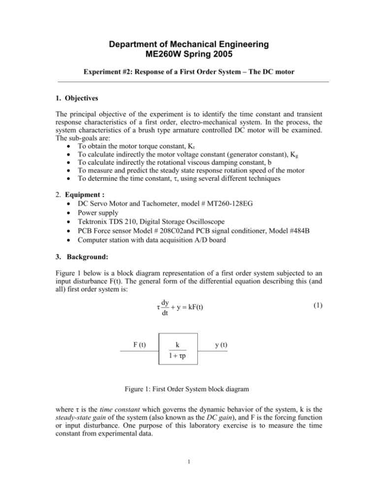
Department of Mechanical Engineering
ME260W Spring 2005
Experiment #2: Response of a First Order System – The DC motor
1. Objectives
The principal objective of the experiment is to identify the time constant and transient
response characteristics of a first order, electro-mechanical system. In the process, the
system characteristics of a brush type armature controlled DC motor will be examined.
The sub-goals are:
 To obtain the motor torque constant, Kt
 To calculate indirectly the motor voltage constant (generator constant), Kg
 To calculate indirectly the rotational viscous damping constant, b
 To measure and predict the steady state response rotation speed of the motor
 To determine the time constant, , using several different techniques
2. Equipment :
 DC Servo Motor and Tachometer, model # MT260-128EG
 Power supply
 Tektronix TDS 210, Digital Storage Oscilloscope
 PCB Force sensor Model # 208C02and PCB signal conditioner, Model #484B
 Computer station with data acquisition A/D board
3. Background:
Figure 1 below is a block diagram representation of a first order system subjected to an
input disturbance F(t). The general form of the differential equation describing this (and
all) first order system is:
τ
F (t)
dy
 y  kF(t)
dt
(1)
y (t)
k
1  τp
Figure 1: First Order System block diagram
where τ is the time constant which governs the dynamic behavior of the system, k is the
steady-state gain of the system (also known as the DC gain), and F is the forcing function
or input disturbance. One purpose of this laboratory exercise is to measure the time
constant from experimental data.
1
Consider the response of a system described by equation (1) to a step-input disturbance.
The forcing (or input) function is given as:
F(t)  X u(t)
(2a)
where X is a constant and u(t) is the Heaviside step function given by
0
u(t)  
1
for t  0
for t  0
(2b)
The response to this input is:
t
y(t)  Y 1  e τ 


where the steady-state response magnitude is given by Y = k X (k = DC gain).
(3)
 will be extracted in three different ways:
1) The step response of the system is shown in Figure 2. Several key aspects of the
response are also labeled. The first of these aspects is referred to as the 63.2% response
point, which is obtained when t/τ = 1. This is the point where;
y(t  τ)
 (1  e 1 )  0.632
(4)
Y
This means that the response y(t) is at 63.2% of the final steady-state value Y. Thus, the
time constant can be quickly determined, if the point at which the response at 63.2% of
its steady-state value is estimated quickly.
1
0.9
0.8
y(t)/Y
0.7
0.632
0.6
0.5
0.4
0.3
0.2
t1
τ
0.1
0
0
1
t/
t1
1
τ
2
Figure 2: Step response of a first order system
2
3
2) The time constant of the system can also be identified by calculating the slope of the
response, i.e. the derivative of the response with respect to time. Taking the derivative of
the response (equation (3)) yields an expression for the slope of the response at any given
time:
dy Y  t τ
 e
dt
τ
(5)
This slope can be used to write an expression for a line tangent to the curve at any point
in time. This tangent line has the form


- t1
y(t)  Y1 - e 

  Y  t1 τ
 e
 τ
 

(t  t 1 )


(6)
where t1 is the time at which the tangent line is drawn. As illustrated in Figure 2, the
tangent intersects with the steady-state value Y at a time,  sec later
t  t1  τ
(7)
This provides a second means for evaluating the time constant, as this behavior is
common to all first order systems. In other words, if the slope of the response curve at
any arbitrary time is extrapolated to intersect with the asymptotic response, the
intersection will take place  time units after the point the tangent was taken.
These two methods, the 63.2% response point and tangent intersection point, are two
quick ways to estimate the time response of the system.
3) If the experimental data are scattered, or if the steady-state value is unknown it may be
difficult to identify the 63.2% response point. Taking the derivative of the response to
evaluate the time constant via the intersection method is also prone to problems, because
experimental slopes will be highly sensitive to variations in data. A more rigorous way to
determine the time constant is to perform linear regression on the data. This is
accomplished by rearranging equation (3) as:
y(t)
t
e τ
Y
Taking the natural log of both sides will result in an equation that is linear in time:
1-
1
 y(t) 
ln 1 
 t

Y 
τ

(8)
(9)
Considering time as the independent variable and the entire left-hand side as the
dependent variable, this is a linear relationship that can be used to determine the time
constant via linear regression. After the transformation, the data will fall on a straight line
as shown in Figure 3. When the data is treated in this manner, the fitted line is
constrained to pass through the origin (since there is only one fitting constant!) and has a
slope equal to the reciprocal of the time constant.
3
t
0
ln(1-y/Y)

1
τ
1
Modeling
a DC
Figure
3: Semioflog
plotMotor
of theSystem
step response
An armature controlled DC motor is given schematically in Figure 4. An input voltage, ei,
is provided by an external power supply. The motor possesses an internal resistance, R,
and an inductance, L. This inductance is a result of the electromagnetic effect developed
by the armature windings, and has a negligible effect for most times of interest. The shaft
of the motor and driven component (a disk in the present lab) have an inherent rotational
inertia, J. The system also experiences viscous damping, characterized by the coefficient
b, due to internal and air damping.
A mathematical model of this motor can be developed by considering the electrical and
mechanical constituents of the system separately. The following equation describes the
armature circuit:
ei  R i  K g Ω
(10)
where ei is the voltage applied to the armature, R is the resistance of the windings, i is the
current, Kg is the motor voltage constant (or generator constant) and Ω is the angular
velocity of the motor shaft. The last term of equation (10) is commonly called the back
emf developed within the motor - it is a reverse voltage proportional to the angular speed
of the shaft. (Note: this characteristic is inherent because of the motor's capability to act
as a generator as well as a motor. That is, if the shaft was turned by an alternative source
(e.g. water), the same armature could be used to generate electricity.)
R
ei
L
b
J
ei
T, 
Figure 4: Schematic of the test setup
4
The output torque T developed at the armature shaft is proportional to the armature
current, i.e.
(11)
T  Kt i
This provides a connection between the mechanical response of the set-up and the
electrical behavior of the motor. (The two motor constants, Kt, and Kg are actually equal
to one another, though details of this connection will not be presented here.) In this
particular set-up, the output torque is used to overcome the motor inertia and frictional
drag. If the frictional drag is viscous in nature, the equilibrium equation of the rotor
system is:
dΩ
TJ
 bΩ
(12)
dt
where J is the inertia of the rotating parts, and b is the rotational viscous damping
coefficient. A composite block diagram of equations (10)-(12) is shown in Figure 5. The
symbol p is the differential operator and is equivalent to differentiation with respect to
time.
Thus, the input to this system is the voltage potential ei applied to the armature, and the
response is the angular velocity Ω. Equations (10)-(12) can be combined (eliminating T
and i) to produce one differential equation which describes the combined electromechanical response of the system:
dΩ
τ
 Ω  k ei
(13a)
dt
where the time constant of the system is given by
τ
b
J
KtKg
(13b)
R
and the steady-state gain is given by
k
ei
+
-
1
(13c)
bR
Kg 
Kt
1
R
Kt
Kg
Fig. 5: A simplified block diagram
5
1
Jpb

R’
R
b
Motor
ei
Tachometer
e0 =K
J
Load
To x-y plotter
Figure 6: Free rotation test
Equation (13a) is a first order differential equation in the standard form. The time
constant τ is representative of the response speed of the system, and the gain constant k
dictates the steady-state sensitivity behavior between the system output and input.
5. General Strategy for Parameter Evaluation:
In order for the above equations to be utilized in simulating the system, it is necessary to
collect sufficient data to determine the system parameters, e.g. Kt, b, Kg, etc. In this
section, a general strategy for obtaining the system parameters is outlined. A detailed
procedure is given in the subsequent section.
Block rotor test (to determine Kt):
If the motor armature is locked (i.e. prevented from rotating) and a voltage potential ei is
applied, the output torque is still related to the armature current by Equation (11). The
armature current can be varied by introducing additional resistances in series into the
armature circuit, as shown in Figure 6. The corresponding motor torque is measured by a
suitably mounted force transducer. The motor torque constant Kt is obtained by plotting
the output torque vs. current (T vs. i) data. The slope is Kt.
CAUTION: In order to not burn out the armature windings, it is important to obtain the
experimental data as quickly as possible.
Free speed test (to determine Kg and b):
Recall that the gain constant is simply a ratio of the output speed to input voltage:


ei
1
bR
Kg 
Kt
.
(13c)
Furthermore, this gain depends on the resistance of the circuitry involved. Using a single
resistor in series with the internal resistance of the motor, the steady state speed can be
6
measured (recall that ei = 24 volts in all cases). Substituting the known values for R, Kt,
ei, and the measured output  into equation (13c) leaves one equation for two unknowns
(Kg and b). Using a different resistor in the circuit will produce a different steady state
rotation speed. Substituting these new values into equation (13c) gives a second equation
for the same two unknowns. A more graphical approach is to rewrite equation (13c) as
 b 
ei
 R.
 K g  
(14)

 Kt 
Plotting the aforementioned data using this equation it becomes evident that the intercept
is Kg, the motor constant. Also, the slope is a combination of b and Kt. This is shown
graphically in Figure 7.
ei

b
1
Kt
Kg
0
R
Figure 7: Test for determining b & Kg
Transient test:
The differential equation that describes the behavior of the DC motor is of first order.
Measuring the time constant of the system, will be accomplished using the three
techniques described in section 3. Furthermore, once the time constant is determined, the
rotary inertia to be determined by rearranging the Equation (13b);
 Kt Kg 
J  τ b 1 

bR 

5. Experimental Procedure:
The overall experimental setup is shown schematically in Figure 8.
7
(15)
DC Motor
SCXI Chassis Power Supply
Signal
Conditioner
Computer
Figure 8: Experimental Apparatus
Blocked Rotor Test
Unhook the wires running from the power supply to the motor. Using a digital
multimeter, verify that the input voltage is 24 volts. With the same multimeter, measure
the internal resistance across the motor. Reattach the motor to the power supply.
Attach the moment arm to the load (the disk), and bring it into contact with the force
transducer such that it blocks the armature from rotation. The PCB power supply for the
force transducer should be adjusted to have a gain of 1 (see back of the power supply).
Rotate the armature away from the force transducer and adjust the dial indicator on the
front of the PCB power supply, until the load recorded by LabView is zero. This zeros
out the force transducer. Rotate the disk until the armature once again contacts the force
transducer. With no external resistance in the armature circuit (flip the switch to 0 ohms),
turn on the circuit and record the resulting torque (this is done in LabView). This test
should be carried out as quickly as possible to avoid overheating of the motor. Note
that the force transducer actually puts out a voltage. However, there is a supplier provided
calibration constant between the output voltage and the force. Multiplying this force by
the moment arm of the armature gives the resulting torque. This is all done internally for
you in the LabView routine.
The current supplied to the motor may be calculate using
i
ei
R
(16)
where ei and R are known. Knowing the supplied current and the output torque, the motor
constant Kt may be determined using equation (11).
Free Speed Test
Carefully disengage the moment arm from the load. With no external resistance in the
circuit (leave the switch at 0 ohms), apply DC power to the circuit and wait until the
motor reaches its steady-state speed. Record this speed. Turn the power supply off and
let the motor come to a stop. Now add a 1-ohm resistor in series with the motor resistance
by flipping the resistance switch to “1 ohm”. Start the motor up again and allow it to
come to steady state. Record this new rotation speed. Knowing the values of the steady
8
state speed and the additional resistance, equation (14) may be used to determine the
unknown motor generator constant Kg and the viscous damping constant b. Repeat this
procedure several times and create a plot similar to that shown in Figure 7. Compare your
Kg with your Kt obtained from the blocked motor test, both in value and in units. Discuss
the reasons if they are different.
Transient test
Record the transient time response of the motor during start-up. Do this test twice – once
having no resistor in series with the motor and once with the 1 ohm resistor in series with
the motor. From these results, determine the time constant of the system using the three
methods described previously. Also determine the net moment of inertia of the system.
Note that the mass moment of inertia of the combined system is made up of the motor
armature, the tachometer armature and the installed rotor.
7. Acquiring Test Data using LabView
Exercise 1: Block rotor test (to determine motor torque constant Kt):
In this exercise, the force1102.VI is used to determine the motor stall torque. The
force1102.VI front panel is shown in Figure A1. After setting the parameters on the front
panel of the VI, attach the moment arm to the flywheel, and bring it to contact the force
transducer such that it blocks the armature from rotation. Set the DC power supply to 24
volts and leave this setting through the entire test sequence. With no external resistance in
the armature circuit, turn on the circuit and recording the resulting force. Use the data
acquisition system and run the force1102VI. After sampling the signal from the
accelerometer for a predetermined length of time, the sampled signal is displayed and the
resulting force and the corresponding voltage can be found.
Make sure your workstation is set up in the following manner:
1. Open the VI. (c:\me260w\lab5 _SDOF lab\force1102.vi)
2. Make sure the SCXI chassis is turned on.
3. Press the Save data button on the VI front panel (Option). This stores the data in
a file.
4. Set the following parameters on the VI:
 Sample rate: as desired (e.g.1024)
 Samples: as desired (e.g. 1024)
 Device:1
 Channels :ob0!sc1md2!0
5. Run button in the top left corner of the VI.
9
Exercise 2: Free speed test (to determine the motor generator constant Kg and the
viscous damping constant b):
Carefully disengage the moment arm from the load. With no external resistance in the
circuit, apply DC power to the circuit and wait until a steady-state speed of the motor is
obtained. Repeat this test for various armature resistances. Calculate the resulting gain
constant k.
The rpm 1102.VI lets you measure motor rpm and the tachometer voltage. Figure 2A is
the front panel of the rpm1102.VI. The steps required for taking a tachometer voltage
measurement are provided. Read through them carefully and do not be afraid to try things
on the device. If you have a question after trying things on your own, contact your
instructor.
Taking Measurements:
Make sure your workstation is set up in the following manner:
1. Open the VI. (c:\me260w\lab5_SDOF lab\rpm1102.vi)
2. Make sure the SCXI chassis is turned on.
3. Press the Save data button on the VI front panel (Option). This stores the data in an
array.
Set the following parameters on the VI:

Device: 1

Channels: ob0!sc1md2!0:1

Sample rate: as desired (e.g. 10240)

Scans: as desired (e.g. 10240)

Filter: on

Filter type: low pass (select it only if the filter is ON)

Windows: None

Filter type: select as desired (non, low pass filter, high pass filter, band pass)

Low cut off: 20

High cut off: 50
4. Run button in the top left corner of the VI.
10
1st Order Motor Tests
number of samples
sample rate
1000.00
Plot 0
Voltage
channel (0)
device
Save
1
1
5000
OFF
Plot 0
Force
0.3
5.0
4.5
4.0
3.5
0.2
3.0
2.5
2.0
0.1
1.5
1.0
0.5
0.0
0.0
0.0
0.5
1.0
1.5
2.0
2.5
3.0
3.5
4.0
4.5
sec
5.0
0.0
0.5
1.0
1.5
2.0
Cursor 0
0.34
0.08
Cursor 0
0.52
17.61
Cursor 1
0.00
-0.01
Cursor 1
0.34
0.00
Figure A1: The force1102.VI front panel.
SDOF LAB2
Figure A2: The rpm1102.VI front panel.
11
2.5
3.0
3.5
4.0
4.5
sec
5.0