Chi-Square Test for Trend in Binomial Proportions in (2 x k) Tables
For test details and example see pages 430-437 in your text. The test itself is certainly
doable by hand, but why? Learning to program R is a worthwhile endeavor as it allows
you to program non-standard test procedures yourself.
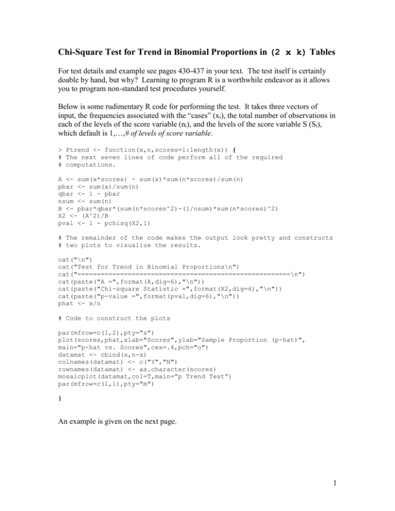
Below is some rudimentary R code for performing the test. It takes three vectors of
input, the frequencies associated with the “cases” (xi), the total number of observations in
each of the levels of the score variable (ni), and the levels of the score variable S (Si),
which default is 1,…,# of levels of score variable.
> Ptrend <- function(x,n,scores=1:length(x)) {
# The next seven lines of code perform all of the required
# computations.
A <- sum(x*scores) - sum(x)*sum(n*scores)/sum(n)
pbar <- sum(x)/sum(n)
qbar <- 1 - pbar
nsum <- sum(n)
B <- pbar*qbar*(sum(n*scores^2)-(1/nsum)*sum(n*scores)^2)
X2 <- (A^2)/B
pval <- 1 - pchisq(X2,1)
# The remainder of the code makes the output look pretty and constructs
# two plots to visualize the results.
cat("\n")
cat("Test for Trend in Binomial Proportions\n")
cat("=======================================================\n")
cat(paste("A =",format(A,dig=6),"\n"))
cat(paste("Chi-square Statistic =",format(X2,dig=6),"\n"))
cat(paste("p-value =",format(pval,dig=6),"\n"))
phat <- x/n
# Code to construct the plots
par(mfrow=c(1,2),pty="s")
plot(scores,phat,xlab="Scores",ylab="Sample Proportion (p-hat)",
main="p-hat vs. Scores",cex=.4,pch="o")
datamat <- cbind(x,n-x)
colnames(datamat) <- c("Y","N")
rownames(datamat) <- as.character(scores)
mosaicplot(datamat,col=T,main=”p Trend Test”)
par(mfrow=c(1,1),pty="m")
}
An example is given on the next page.
1
Example: Breast Cancer and Age at 1st Birth (see pg. 433)
>
>
>
>
x <- c(320,1206,1011,463,220)
n <- c(1742,5638,3904,1555,626)
scores <- c(1,2,3,4,5)
Ptrend(x,n,scores)
Test for Trend in Binomial Proportions
=======================================================
A = 567.16
Chi-square Statistic = 129.012
p-value = 0
2