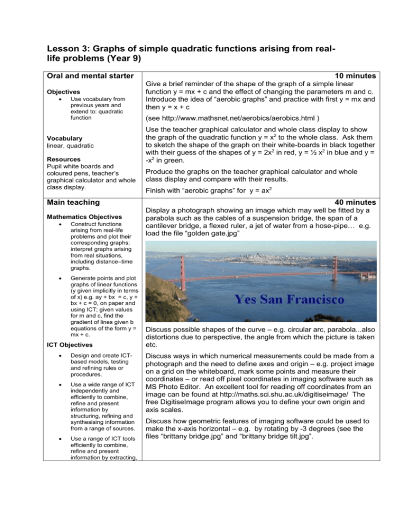
Lesson 3: Graphs of simple quadratic functions arising from reallife problems (Year 9)
Oral and mental starter
Objectives

Use vocabulary from
previous years and
extend to: quadratic
function
Vocabulary
linear, quadratic
Resources
Pupil white boards and
coloured pens, teacher’s
graphical calculator and whole
class display.
Main teaching
Mathematics Objectives

Construct functions
arising from real-life
problems and plot their
corresponding graphs;
interpret graphs arising
from real situations,
including distance–time
graphs.

Generate points and plot
graphs of linear functions
(y given implicitly in terms
of x) e.g. ay + bx = c, y +
bx + c = 0, on paper and
using ICT; given values
for m and c, find the
gradient of lines given b
equations of the form y =
mx + c.
ICT Objectives

Design and create ICTbased models, testing
and refining rules or
procedures.

Use a wide range of ICT
independently and
efficiently to combine,
refine and present
information by
structuring, refining and
synthesising information
from a range of sources.

Use a range of ICT tools
efficiently to combine,
refine and present
information by extracting,
10 minutes
Give a brief reminder of the shape of the graph of a simple linear
function y = mx + c and the effect of changing the parameters m and c.
Introduce the idea of “aerobic graphs” and practice with first y = mx and
then y = x + c
(see http://www.mathsnet.net/aerobics/aerobics.html )
Use the teacher graphical calculator and whole class display to show
the graph of the quadratic function y = x2 to the whole class. Ask them
to sketch the shape of the graph on their white-boards in black together
with their guess of the shapes of y = 2x2 in red, y = ½ x2 in blue and y =
-x2 in green.
Produce the graphs on the teacher graphical calculator and whole
class display and compare with their results.
Finish with “aerobic graphs” for y = ax2
40 minutes
Display a photograph showing an image which may well be fitted by a
parabola such as the cables of a suspension bridge, the span of a
cantilever bridge, a flexed ruler, a jet of water from a hose-pipe… e.g.
load the file “golden gate.jpg”
Discuss possible shapes of the curve – e.g. circular arc, parabola...also
distortions due to perspective, the angle from which the picture is taken
etc.
Discuss ways in which numerical measurements could be made from a
photograph and the need to define axes and origin – e.g. project image
on a grid on the whiteboard, mark some points and measure their
coordinates – or read off pixel coordinates in imaging software such as
MS Photo Editor. An excellent tool for reading off coordinates from an
image can be found at http://maths.sci.shu.ac.uk/digitiseimage/ The
free DigitiseImage program allows you to define your own origin and
axis scales.
Discuss how geometric features of imaging software could be used to
make the x-axis horizontal – e.g. by rotating by -3 degrees (see the
files “brittany bridge.jpg” and “brittany bridge tilt.jpg”.
combining and modifying
relevant information for
specific purposes.

Use ICT to draft and
refine a presentation,
including capturing still
and moving images (e.g.
using a scanner, digital
camera, microphone),
and importing and
exporting data and
information in appropriate
formats.
Vocabulary
parabola, quadratic function,
axes, origin, perspective,
translation, scale, vertex,
symmetry, scatter graph,
model
Now measure coordinates of important points from the image –
commenting on appropriate accuracy and units. With DigitiseImage
you can define O as origin, say, and units on the x- and y-axis of 300
pixels to export co-ordinate data for the marked points:
Resources
PC with data-projector and
white-board, class set of
graphical calculators, teacher’s
graphical calculator and whole
class display, resource sheets
M3 and H3, image files.
In MS Photo Editor the points marked A, B, D, C have approximate
pixel values: (121,95), (122,138), (486, 83), (485, 135). Transform
these into approximate pixel displacements from an origin O:
(-180, 45), (-180, 0), (0, 0), (180, 0), (180, 45)
and rescale into simpler units e.g. 1 unit = 45 pixels
(-4, 1), (-4, 0), (0, 0), (4, 0), (4, 1)
Enter the x- and y-coordinates of A, O and D into the lists of the
graphical calculator, draw a scatter graph, choose suitable axes and
then fit different models of y = ax2 to the data. Project the graphical
calculator display to superimpose over the image (or a sketch taken
from it).
(An alternative approach is to use dynamic geometry software to
superimpose axes and the graph of a function directly over an image –
see The Geometer’s Sketchpad file “Britanny bridge.gsp”.)
Now give pupils the pupil sheet from which to measure and record
coordinates, draw a scatter graph and fit a quadratic function.
Plenary
By the end of the lesson
pupils should be able to explain
how to find, calculate and use:

Be able to generate
points and plot the
graphs of simple
quadratic or cubic
functions using ICT.
10 minutes
Discuss principal features of parabolas and quadratic functions –
symmetry, vertex, axis….Discuss where parabolas may occur in nature
– bridge types, arches, water spouts, lenses …
Homework:
Find good websites with images of bridges or other parabolic objects
(e.g. use a search engine with “bridges pictures parabola”…)
Or:
Use a digital camera to take pictures of a flexed ruler on squared paper
and read off coordinates. Fit a quadratic function.
(Pupils without access to Internet or digital camera/PC can draw and
measure without need for ICT!)