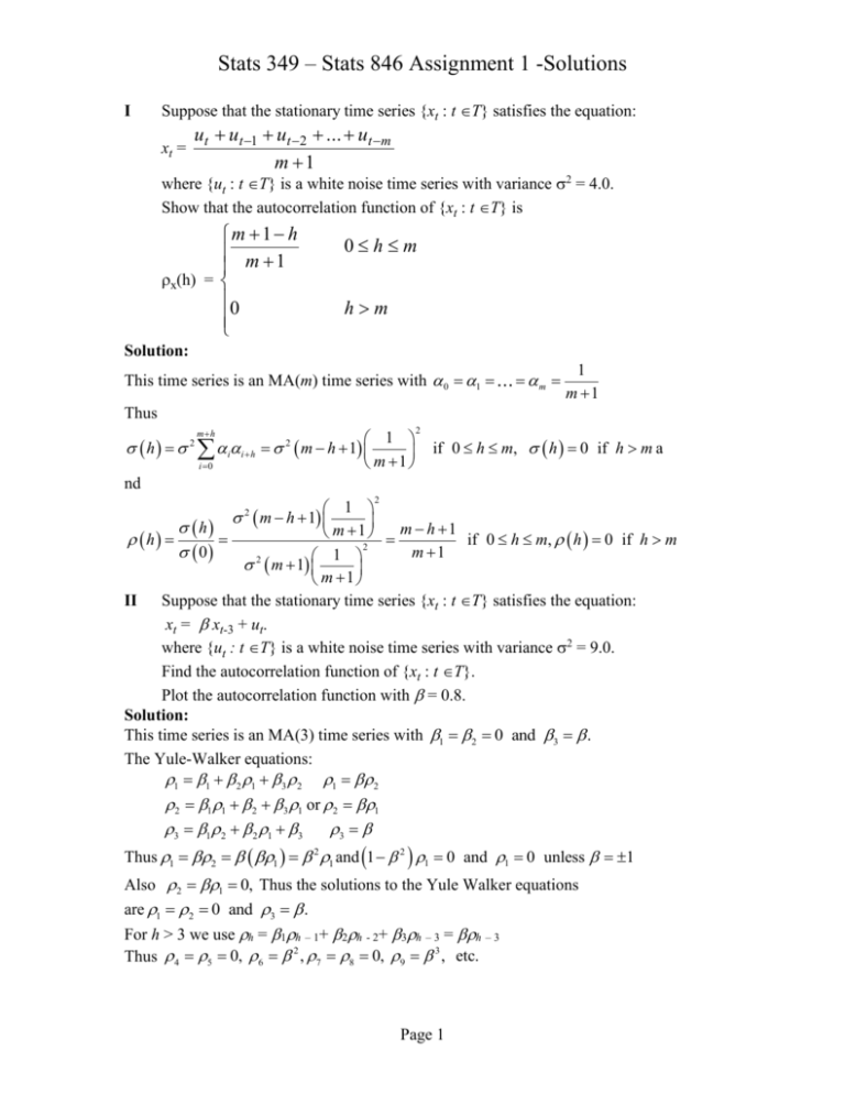
Stats 349 – Stats 846 Assignment 1 -Solutions
I
Suppose that the stationary time series {xt : t T} satisfies the equation:
xt =
ut  ut 1  ut 2  ...  ut m
m 1
where {ut : t T} is a white noise time series with variance 2 = 4.0.
Show that the autocorrelation function of {xt : t T} is
m  1  h
 m 1

x(h) = 
0

0hm
hm
Solution:
This time series is an MA(m) time series with  0  1 
 m 
1
m 1
Thus
 h  
mh
2
 
i 0
i
ih
 1 
   m  h  1 

 m 1 
2
2
if 0  h  m,   h   0 if h  m a
nd
2
 1 

 h
 m  1   m  h  1 if 0  h  m,  h  0 if h  m
 h 

 
2
  0
m 1
 1 
2
  m  1 

 m 1 
II Suppose that the stationary time series {xt : t T} satisfies the equation:
xt =  xt-3 + ut.
where {ut : t T} is a white noise time series with variance 2 = 9.0.
Find the autocorrelation function of {xt : t T}.
Plot the autocorrelation function with = 0.8.
Solution:
This time series is an MA(3) time series with 1   2  0 and 3   .
The Yule-Walker equations:
1  1   2 1  3  2 1   2
 2  m  h  1 
 2  11   2  3 1 or 2  1
3  1 2   2 1  3
3  
Thus 1  2    1    2 1 and 1   2  1  0 and 1  0 unless   1
Also 2  1  0, Thus the solutions to the Yule Walker equations
are 1  2  0 and 3   .
For h > 3 we use h = 1h – 1+ 2h - 2+ 3h – 3 = h – 3
Thus 4  5  0, 6   2 , 7  8  0, 9   3 , etc.
Page 1
Stats 349 – Stats 846 Assignment 1 -Solutions
Plot of autocorrelation function:
1.2
1
0.8
0.6
0.4
0.2
40
38
36
34
32
30
28
26
24
22
20
18
16
14
12
10
8
6
4
2
0
0
III. Consider the Autoregressive (AR(3)) process of order 3 satisfying the equation:
xt= 1xt-1 + 0.25xt-2 - 0.10xt-3+  + ut where var(ut) = 2.
Suppose that the autocorrelation function, (h), at lag h = 1 takes on the values
(1) = 0.50. In addition var(xt) = 10 and E[xt] = = 25
a) Determine the values of 1,  and 2 .
Solution This is an AR(3) time series with 1 (unknown), 2 = 0.25 and 3 = 0.10.
The Yule-walker equations are
0.5  1   0.25 0.5   0.10  2
1  1   2 1  3  2
 2  11   2  3 1 or 2  1  0.5   0.25   0.10  0.5
3  1 2   2 1  3
3  12   0.25 0.5   0.10 
The first two equations can be used to solve for 1 and 2.
1  0.375  0.102 and 2  0.51  0.30  0.5 0.375  0.10 2   0.30
0.4875
 0.46429
1.05
and 1  0.375  0.102  0.375  0.10  0.46429  0.32857
1.05 2  0.5  0.375   0.30  0.4875 and  2 
Finally 25   





 1   2  3  0.32857  0.25  0.10 0.32143
and    0.32143 25  8.036
Now 1  0.5, 2  0.46429 . The third equation of the Yule-Walker equations can be
used to calculate 3. Namely
3  12  2 1  3   0.32857  0.46429   0.25 0.50   0.10  0.377551
Page 2
Stats 349 – Stats 846 Assignment 1 -Solutions
To compute 2 we use
10.0    0  

2
1  1 1   2 2  3 3
2
1  0.32857 .5   0.25  0.46429   0.10  0.377551

2
0.681888
Thus   10.0 0.681888  6.81888
2
b) Compute and plot a graph of (h), the auotocovariance function of the process
at lag h, for h = 0, 1, 2, 3, 4.
Solution:
For h >3 we use h  1h1  2 h2  3 h3  0.32857 h1  0.20h2  0.10h3
Thus 4  0.32857  0.377551  0.25  0.46429  0.10  0.5  0.290124
Finally
The autocovariance function is determined by (h) = (0) h= 10.0 h
Thus (0)=10.0, (1) = 5.0, (2) = 4.6429, (3) = 3.77551, (4) = 2.90124
IV.
An AR(2) time series, {xt : t T}, if | r1 | >1 and | r2 | >1, where r1 and r2 are the
roots ofthe polynomial 1 -1 x - 2x2 = 0. Show that an AR(2) time series is
stationary if the parameters, 1 and 2, satisfy the following inequalities:
2 + 1 < 1,
2 - 1 < 1,
-1 < 2 < 1.
2
Show that roots r1 and r2 are complex if 1+ 4 2 < 0.
Graph this regions implied by these inequalities.
Solution:
 x 
1 1  1  2
x
1  1 x   2 x 2  1  1    1     x  
 x where
 r1  r2 
 r1 r2   r1r2 
1    4 2
r1 , r2 
are the roots of 1  1 x   2 x 2
2 2
Note: r1 , r2 are complex if   4 2  0 Also 1 
1 1
1
1

and  2  
, , 2 
r1 r2
r1r2
r1 r2
1 1 1  1  1 
 
 1  1  
r1 r2 r1r2  r1  r2 
1 1 1  1  1 
and 1   2  1  1   
 1  1  
r1 r2 r1r2  r1  r2 
1
Now  2 
 1 , 1  1   2  0 and 1  2  1  0 if and only if r1  1 and r2  1
r1 r2
Thus 1  1   2  1 
Page 3