DERIVATIVES AND OPTIMIZATION
© 2011, Kwan Choi.
Since marginal concepts are ubiquitous in most economic problems, we consider
derivatives in this note. You have been exposed to the derivatives already. You are
familiar with the notions of marginal costs, marginal products, marginal utilities,
etc. There are many derivative rules or formulas which you could learn from any
calculus course. To get through the basic optimization concepts, we will consider
the most widely used formula, the one for polynomials.
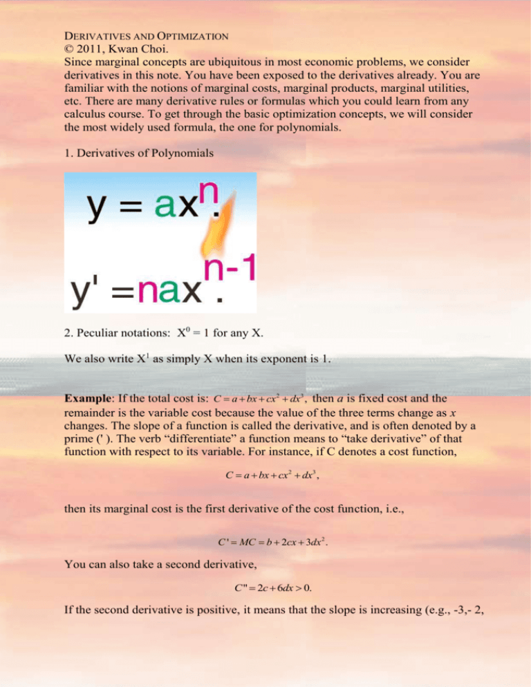
1. Derivatives of Polynomials
2. Peculiar notations: X0 = 1 for any X.
We also write X1 as simply X when its exponent is 1.
Example: If the total cost is: C  a  bx  cx2  dx3 , then a is fixed cost and the
remainder is the variable cost because the value of the three terms change as x
changes. The slope of a function is called the derivative, and is often denoted by a
prime (' ). The verb “differentiate” a function means to “take derivative” of that
function with respect to its variable. For instance, if C denotes a cost function,
C  a  bx  cx 2  dx3 ,
then its marginal cost is the first derivative of the cost function, i.e.,
C '  MC  b  2cx  3dx 2 .
You can also take a second derivative,
C "  2c  6dx  0.
If the second derivative is positive, it means that the slope is increasing (e.g., -3,- 2,
-1, 0, 1, 2, 3) as x increases, and hence it has a minimum. If the second derivative
is negative, the slope is declining (e.g., 3, 2, 1, 0, -1, -2, -3), it has a maximum.
Partial Derivatives
Sometimes there are two or more control variables to manipulate the objective
function (profit function, utility function, cost function, etc.) If there are two
variables, X and Y, it is necessary to distinguish the partial derivative with respect
X and Y.
For instance, there are many consumption goods, it is necessary to distinguish
marginal utilities of different goods. For instance, marginal utility of good 1 is the
increment of utility attained from an extra unit of that good, holding the quantity
of the other good (the quantities of all other goods) constant. Marginal utility of X 1
is written as:
MU X 
2
U
.
X
Note that units of measurement are arbitrary. Hence, marginal utilities of the same
good can differ if the extra units are measured in gram or kilogram or pound. It is
often useful to measure marginal utilities when the extra unit becomes extremely
small, or infinitesimally small.
In Figure 14, marginal utility is the slope of the line AB. However, as ΔX becomes
infinitesimally small or approaches zero, line AB approaches the tangent line AD.
For practical reasons, it is safe to argue that marginal utility is the slope of the
tangent line AD (at the consumption point A).
Marginal utilities are measured while all other goods are held constant. Thus,
marginal utility of X is a partial derivative of U with respect to X. The quantities
of all other goods are held constant.
MU X 
dU
U U
 lim

.

x

dX
X X
Example:
Let
U ( X , Y )  XY
be the utility function.
A partial derivative with respect to X ignores all variables other than X and treat
them as if they are constant.
Derive marginal utilities of X and Y when evaluated at X = 5, and Y = 7.
MU X 
U
 Y  7,
X
(1)
MU Y 
U
 X  5.
Y
(2)
Derive the marginal utilities of X and Y when U ( X , Y )  X 1/ 3Y 2/ 3 .
2
1 2 2 1  Y 3
MU X  X 3Y 3    .
3
3 X 
3
(3)
1
2 13  13 2  X  3
MUY  X Y    .
3
3 Y 
(4)
Marginal Rate of Substitution
Along a given indifference curve, consumption of two goods can be changed
without altering the utility level. This means that on an indifference curve, the
change in utility is zero.
dU 
U
U
dx1 
dx2  MU1dx1  MU 2 dx2  0,
x1
x2
The slope of the indifference curve is the ratio of marginal utilities:

dx2 MU1

.
dx1 MU 2
In Figure 15, marginal rate of substitution (of x 1 for x2) is the slope of the ray AB.
However, here the change in good 1 (Δx1) is rather large. As Δx1 becomes
infinitesimally small or approaches zero, the slope of line AB approaches the
tangent line AD. Thus, for practical reasons, it is safe to say that MRS at point A is
the slope of the indifference curve (at that point).
4
Remark: As Q becomes infinitesimally small, Marginal Cost approaches the slope
of the TC curve. Thus, MC is the slope of the TC or its derivative, dC / dX .
Unconstrained maximization problem
The Single Variable Case
Choose x to maximize the objective function (x).
The First Order Condition (FOC): The first derivative must be zero at the
maximum or minimum,
d
  '( x)  0.
dx
The Second Order Condition (SOC): The second derivative must be negative for a
5
maximum, and positive for a minimum.
 "( x)  0.
Multivariate Case
Choose X and Y to maximize  ( X , Y ).
The First order condition (FOC): Each partial derivative must be zero. That is,

 0,
X

Y 
 0.
Y
X 
The Second order condition (SOC): Each second order derivative must be negative
(  XX  0,  YY  0 ), but also  XX  YY   XY 2  0. For a minimum, each second order
derivative must be positive (  XX  0,  YY  0 ), and  XX  YY   XY 2  0. If the latter
condition is not satisfied, i.e., if  XX  YY   XY 2  0, then it is a saddle point.
EXAMPLE
Let
Y  F ( K , L)  AK 1/ 3 L2/ 3
(5)
be a production function. Derive MRTS.
Along an isoquant, the output level is fixed, i.e., dY = 0. Totally differentiating (5),
we get
FK dK  FL dL  0,
(6)
where Fi  F / i is marginal product of input i. Thus, the slope of an isoquant is

dK FL

.
dL FK
(7)
Note
FK  F / K 
6
A 2 / 3 2 / 3
K L .
3
(8)
FL  F / L 
2 A 1/ 3 1/ 3
K L .
3
(9)
Substituting (8) and (9) into (7), we get marginal rate of technical substitution
(MRTS) of capital (K) for labor (L):
MRTS 
2K
.
L
(10)
Constrained Minimization Problem
The firm’s cost minimization problem is to choose K and L to
Minimize C  wL  rK , (cost)
Subject to y  f ( K , L)  0. (output constraint)
The Lagrangian function associated with this problem can be written as:
L  wL  rK  [ y  f ( K , L)].
(11)
The first order conditions are:
L
 r   f K  0,
K
(12)
L
 w   f L  0,
L
(13)
L
 y  f ( K , L)  0,

(14)
where the subscripts denote partial derivatives, i.e., f / K  f K and f / L  f L .
From the two equations in (13) and (14), we get

w
r

.
fL fK
Rearranging this, we obtain
MRTS KL 
fL w
 ,
fK r
(15)
which is the equilibrium condition for cost minimization. Moreover, the value of
the Lagrange multiplier in equilibrium is
7

L C

 MC.
y y
(16)
That is, the Lagrange multiplier is marginal cost of production.
Democracy and Tyranny
The Lagrange multiplier in a constrained optimization problem can be interpreted
as the relative weight or trade-off between two or more competing goals. In the
above example, marginal cost is the trade-off between output and cost. If there are
two industries, efficiency is achieved when one industry’s revenue is maximized
for any given revenue (or output) of the other industry. For instance, a country may
maximize revenue of the private sector for given revenue (or output) of the military
sector (resources are given). In this case, the Lagrangian problem is L  1   2 ,
and  is the weight assigned to the revenue in the defense sector. If  = 0 or close
to zero, it means that the society assigns a low weight to national defense, i.e., little
or no money is spent on national defense.
Next, consider consumer welfare in a society that consists of two or more
8
individuals or regions (Shiites, Kurds, and Sunnis, for example). The Lagrangian
problem can be written as L  u1 ( x)  u 2 ( x), where x is consumption goods, and u1
and u 2 are utilities of consumers 1 and 2, respectively. Intuitively, this problem
maximizes the welfare of individual 1 while guaranteeing a minimum utility ( u 2 )
for individual 2. Of course, this minimum guaranteed utility level for individual or
group 2 can be raised. This amounts to raising the value of . The higher the
minimum guaranteed level of utility, the larger the value of .
In a society with more than two groups, the Lagrangian problem is to maximize
group 1’s welfare, given that some minimum levels of utilities for group 2 and 3
are guaranteed. Thus, the Lagrangian problem is written as:
L  u1 ( x)  2u 2 ( x)  3u 3 ( x)  ...
where i is the Lagrange multiplier for group i.
In extreme cases where i is either zero or near zero, that man’s (or region’s)
welfare is ignored. This is the case of dictatorship, tyranny or slavery. This shows
that “if one man is to be absolutely free, then another must become an absolute
slave.”(Urantia Book.) If domestic privacy must be guaranteed absolutely, then no
phone calls of terrorists can be monitored. In a free market economy, the society
often has two or more conflicting goals, in which case the society solves a
constrained optimization problem, assigning different weights to conflicting goals.
When  = 1 for all, the problem has a significant meaning in the society, because
all individuals are assigned the same weights. “If one man craves freedom 
liberty  he must remember that all other men long for the same freedom.” Thus,
in an ideal society, all are given equal rights (or opportunities), and  = 1 for all
means democracy. In this case, the society maximizes L  u1 ( x)  u 2 ( x)  u 3  ....
Democracy and the free market, of course, do not equalize incomes of all
individuals, because individuals differ in their abilities, tastes or genetic
endowments. Thus, in a free market where all consumers are treated equal, there
will be income differences among individuals. Market economies make two
adjustments. First, historical experiences show that extreme income inequality is a
destabilizing factor in civilizations. Governments in a free market often recognize
this problem and redistributes income from the rich to the poor by income tax.
Second, criminals and underage individuals are not given the voting rights.
9