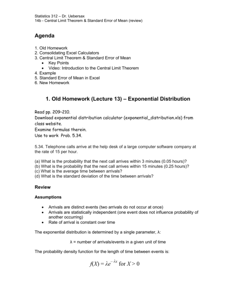
Statistics 312 – Dr. Uebersax
14b - Central Limit Theorem & Standard Error of Mean (review)
Agenda
1. Old Homework
2. Consolidating Excel Calculators
3. Central Limit Theorem & Standard Error of Mean
 Key Points
 Video: Introduction to the Central Limit Theorem
4. Example
5. Standard Error of Mean in Excel
6. New Homework
1. Old Homework (Lecture 13) – Exponential Distribution
Read pp. 209–210.
Download exponential distribution calculator (exponential_distribution.xls) from
class website.
Examine formulas therein.
Use to work Prob. 5.34.
5.34. Telephone calls arrive at the help desk of a large computer software company at
the rate of 15 per hour.
(a) What is the probability that the next call arrives within 3 minutes (0.05 hours)?
(b) What is the probability that the next call arrives within 15 minutes (0.25 hours)?
(c) What is the average time between arrivals?
(d) What is the standard deviation of the time between arrivals?
Review
Assumptions



Arrivals are distinct events (two arrivals do not occur at once)
Arrivals are statistically independent (one event does not influence probability of
another occurring)
Rate of arrival is constant over time
The exponential distribution is determined by a single parameter, λ:
λ = number of arrivals/events in a given unit of time
The probability density function for the length of time between events is:
– λx
f(X) = λe
for X > 0
Statistics 312 – Dr. Uebersax
14b - Central Limit Theorem & Standard Error of Mean (review)
The mean (average) time between events is:
The standard deviation of time between events is:
Cumulative probability:
Pr(arrival time ≤ x) = 1 – e –λx
Answers
λ = 15 (calls per hour)
x = 3 minutes = 3/60 = .05 hours
.
Exponential Distribution Calculator
Statistic
x
lambda (arrival/failure rate)
Pr (X =< x)
Pr (X > x)
mean time between arrivals/failures
std. dev.
Value
0.05
15.0000
0.528
0.472
0.067
0.067
(a) Probability next call arrives within 3 minutes = Pr(X ≤ 0.05) = 0.528
(c) Mean time between arrivals = 0.067
(d) Standard deviation of the time between arrivals = 0.067
(b) Probability next call arrives within 15 minutes (0.25 hours) = 0.976
Statistic
x
lambda (arrival/failure rate)
Pr (X =< x)
Value
0.25
15.0000
0.976
Statistics 312 – Dr. Uebersax
14b - Central Limit Theorem & Standard Error of Mean (review)
2. Demonstration: Consolidating Excel Calculators
This demonstration shows how to consolidate our various individual Excel calculators
into a single file with several worksheets.
3. Review: Central Limit Theorem & Standard Error of Mean
Key Concepts
Sampling. The repeated drawing of samples of some fixed size (n) from a population.
Sampling distribution of the mean. The probability distribution describing the
variability amongst all possible means of size n drawn from a given population.
Standard error (of the mean). The standard deviation of the sampling distribution of the
mean.
Central limit theorem. Let X be a continuous variable with mean μx and standard
deviation σx. Regardless of how X is distributed, the sampling distribution of the mean
formed by taking all possible samples of a given size n will approximate a normal

(Gaussian) distribution with mean
and standard error of the mean


X
  X / n as n increases.
X

X
Statistics 312 – Dr. Uebersax
14b - Central Limit Theorem & Standard Error of Mean (review)
Videos:
jbstatistics playlists:
https://www.youtube.com/user/jbstatistics/playlists
Introduction to the Central Limit Theorem
https://www.youtube.com/watch?v=Pujol1yC1_A
Statistics 312 – Dr. Uebersax
14b - Central Limit Theorem & Standard Error of Mean (review)
4. Example
Refer to jbstatistics video:
Suppose salaries at a large corporation have a mean of $62,000 and a standard
deviation of $32,000.
If 1 employee is randomly selected, what is the probability that their average salary
exceeds $66,000? Answer: We cannot answer this, because we do now know the
shape of the parent distribution (see video).
If 100 employees are randomly selected, what is the probability that their average salary
exceeds $66,000?

X
  X  62000

X
  X / n  32000 / 100  3200
z  (X   X) / X
z = (66000 – 62000) / 3200 = 4000/3200 = 1.25
Cumulative Standard Normal
Distribution (z-to-p)
NORMSDIST()
z
1.2500
p (-inf to z)
0.8944
Pr(z > 1.25) =1 – 0.8944 = 0.1056
Statistics 312 – Dr. Uebersax
14b - Central Limit Theorem & Standard Error of Mean (review)
5. Standard Error of the Mean in Excel
In Lecture 8 you were asked to make an Excel calculator to compute sample/population
variance and standard deviation. Add a new section to this spreadsheet to compute the
standard error of the mean.
That is, add to the existing calculator:
Statistic
Sample variance
Population variance
Sample standard deviation
Population standard deviation
Value
=var(<range>)
=varp(<range>)
=stdev(<range>)
=stdevp(<range>)
the following two rows:
Sample size
Std. error of mean
user supplied
=stdev(<range>)/sqrt(<sample size>)
where <range> is cells that contain raw data (e.g., a:a.) and <sample size> is the
address (or name) of the cell where you have supplied the sample size.
Note: The above corrects an error made in the classroom lecture. You must supply the
sample size (i.e., do not use the population size) for the std. error.
6. New Homework
Download Excel spreadsheet mpg.xls from class website. Suppose the data are
mileage (miles per gallon) from a fleet of 89 utility vans. Treat as a population. For these
data, calculate and report:
1. The population mean and population standard deviation.
2. The standard error of the mean for samples of n = 4.
3. The standard error of the mean for samples of n = 25.
4. Use your z-to-p calculator to compute the probability that the mean mpg of one
random sample of 4 vans from this fleet would be greater than 26 mpg.
For 1: Calculate using Excel (e.g., mystats.xls)
For 2 and 3: Perform calculations manually (using results of 1); show work and
formulas; check answers using Excel.
For 4: Compute z manually (using results of 2) and show formula. Use z-to-p calculator
to compute answer. It is strongly suggested you draw a picture.