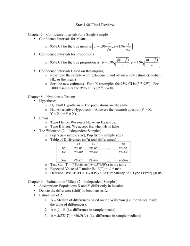
Stat 160 Final Review
Chapter 7 – Confidence Intervals for a Single Sample
 Confidence Intervals for Means

s
s 
o 95% CI for the true mean is  x  1.96
, x  1.96

n
n

 Confidence Intervals for Proportions

pˆ (1  pˆ )
pˆ (1  pˆ ) 

, pˆ  1.96
o 95% CI for the true proportion is  pˆ  1.96

n
n


 Confidence Intervals Based on Resampling
o Resample the sample with replacement and obtain a new estimate(median,
HL, or the mean)
o Sort the new estimates. For 100 resamples the 95% CI is (3rd, 98th). For
1000 resamples the 95% CI is (25th, 976th).
Chapter 8 – Hypothesis Testing
 Hypotheses
o H0: Null Hypothesis – The populations are the same
o HA: Alternative Hypothesis – Answers the research question(Y > X,
Y < X, or Y ≠ X)
 Errors
o Type I Error: We reject H0, when H0 is true.
o Type II Error: We accept H0, when H0 is false.
 The Wilcoxon (2 – Independent Samples)
o Pop Y(n – sample size), Pop X(m – sample size)
o Table of Differences (m*n total differences)
X1
X2
…
Xm
Y1
Y1-X1
Y1-X2
…
Y1-Xm
Y2
Y2-X1
Y2-X2
…
Y2-Xm
…
…
…
…
…
Yn
Yn-X1
Yn-X2
…
Yn-Xm
o Test Stat: T = (#Positives) + 0.5*(#0’s) in the table
o Expected Value of T under H0: E(T) = ½ * m*n.
o Decision: We REJECT H0 if P-Value (Probability of a Type I Error) ≤0.05
Chapter 9 – Estimation of Effect (2 – Independent Samples)
 Assumption: Populations X and Y differ only in location.
 Denote the difference (shift) in locations as 
 Estimation of 
1. ̂  Median of differences based on the Wilcoxon (i.e. the values inside
the table of differences).
2. ̂  y  x (i.e. difference in sample means)
3. ˆ  MED(Y )  MED( X ) (i.e. difference in sample medians)


Confidence Interval for 
o Resample sample Y with replacement and sample X with replacement
o Obtain a new ̂ (by 1, 2, or 3 above)
o Sort the ̂ ’s. For 100 resamples the 95% CI is (3rd, 98th). For 1000
resamples the 95% CI is (25th, 976th).
Difference in independent proportions
o Since a proportion is a mean we can use method 2 above to estimate and
find a 95% CI.
Chapter 10 – Design of Experiments
 Purpose is to establish Cause and Effect
 Completely Randomized Designs
o See Chapter 8 and Chapter 9 for Test Stat, E(T), estimate, and 95% CI
 Randomized Paired Designs
o Randomly Select n Pairs(ID Twins, Yourself, etc.). Apply T1 to half of
the pair(Pop Y) and T2 to the other half of the pair(Pop X)
o PopY and Pop X are dependent(Within each pair there is a dependency).
o Let D1 = Y1 – X1, D2 = Y2 – X2, …, Dn = Yn – Xn (We now have just 1
sample of differences, the D’s)
o Table of Walsh Averages
D1
D2
…
Dn
D1
(D1+D1)/2
x
x
x
D2
(D2+D1)/2
(D2+D2)/2
x
x
…
…
…
…
x
Dn
(Dn+D1)/2
(Dn+D1)/2
…
(Dn+Dn)/2
n(n  1)
2
Test Stat: W = (#Positives) + 0.5*(#0’s) in the table
n(n  1)
Expected Value of W under H0: E(W) =
4
̂  HL Estimate (i.e. median of the Walsh Averages)
95% CI – Use chapter 7 on the D’s using the HL as the estimate
o Total # of Walsh Averages =
o
o
o
o
Chapter 11 – Regression Second Pass
 CRD – Completely Randomized Design
o Plot Pop X at x = 0 and Pop Y and x = 1.
o LS Fit for yˆ  aˆ  bˆx
 Intercept is the average for Pop X
 Slope is the difference(shift - ̂ ) between Pop Y and Pop X on
average
 95% CI for the slope is (bˆ  1.96 SE , bˆ  1.96 SE )