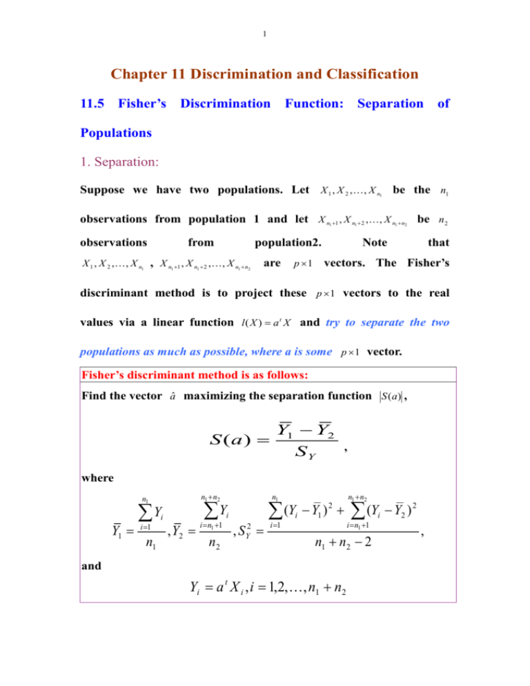
1
Chapter 11 Discrimination and Classification
11.5 Fisher’s Discrimination Function: Separation of
Populations
1. Separation:
Suppose we have two populations. Let X 1 , X 2 , , X n
1
be the n1
observations from population 1 and let X n 1 , X n  2 ,, X n  n be n 2
1
observations
from
1
population2.
X 1 , X 2 ,  , X n1 , X n1 1 , X n1  2 ,  , X n1  n2
are
1
2
Note
that
vectors. The Fisher’s
p 1
discriminant method is to project these p  1 vectors to the real
values via a linear function l ( X )  a t X and try to separate the two
populations as much as possible, where a is some p  1 vector.
Fisher’s discriminant method is as follows:
Find the vector â maximizing the separation function S (a) ,
S (a) 
Y1  Y2
SY
,
where
n1  n2
n1
Y1 
 Yi
i 1
n1
, Y2 
Y
i  n1 1
n2
n1
i
, S Y2 
 (Y  Y )
i 1
i
1
2

n1  n2
 (Y  Y )
i  n1 1
n1  n2  2
and
Yi  a t X i , i  1,2,, n1  n2
i
2
2
,
2
Intuition of Fisher’s discriminant method:
Rp
X 1 , X 2 ,  , X n1
X n1 1 , X n1  2 ,  , X n1  n2
l ( X )  aˆ t X
Yn1 1 , Yn1  2 , , Yn1  n2
Y1 , Y2 , , Yn1
R
Intuitively,
As far as possible by finding â
Y  Y2
measures the difference
S (a)  1
SY
between the
transformed means Y1  Y2 relative to the sample standard deviation
SY
.
If
the
transformed
observations
Y1 , Y2 , , Yn1
and
Yn1 1 , Yn1  2 , , Yn1  n2 are completely separated,
Y1  Y2
should be large as the random variation of the transformed
data reflected by SY is also considered.
Important result:
The vector â maximizing the separation S (a) 
Y1  Y2
SY
is the form
of
1
X 1  X 2 
S pooled
, where
 X
n1
S pooled 
n1  1S1  n2  1S 2 , S
n1  n2  2
n1  n2
S2 
 X
i  n1 1
1

i 1
 X 1 X i  X 1 
t
i
n1  1
 X 2 X i  X 2 
t
i
n2  1
,
,
3
and where
n1  n2
n1
X1 
X
i 1
i
and X 2 
n1
X
i  n1 1
i
n2
.
Justification:
 n1
  Xi
Yi  a X i

t  i 1
i 1
i 1
Y1 

a
 n
n1
n1
 1

n1
n1
t


  at X
1.



Similarly, Y2  a t X 2 . Also,
n1

n1


n1

 (Yi  Y1 )   a X i  a X 1   a t X i  a t X 1 a t X i  a t X 1
2
i 1
t
t
2
i 1

t
i 1
 n1
t
  a X i  X 1 X i  X 1  a  a  X i  X 1 X i  X 1   a .
i 1
 i 1

n1
t
t
t
Similarly,
n1  n2
 Y  Y 
i  n1 1
2
i
2
 n1  n2
t



 a   X i  X 2 X i  X 2 a
i n1 1

t
Thus,
 Y
n1
S Y2 
i 1
i
 Y1  
2
n1  n2
 Y
i  n1 1
i
 Y2 
2
n1  n2  2
 n1  n2
 n1
t
t
a t  X i  X 1 X i  X 1   a  a t   X i  X 2 X i  X 2   a
 i 1

i n1 1


n1  n2  2
4
n1  n2
 n1
t
t
  X i  X 1 X i  X 1     X i  X 2 X i  X 2 
i 1
i  n1 1
 at 

n1  n2  2




a



 n  1S1  n2  1S 2 
t
 at  1
 a  a S pooled a
n1  n2  2


Thus,
Y1  Y2 a t X 1  X 2 
S (a) 

SY
a t S pooled a
â can be found by solving the equation based on the first derivative
of S (a ) ,
2S pooled a
S (a) X 1  X 2  1 t

 a X 1  X 2 
0
3/ 2
t
t
a
2
a S pooled a
a S pooled a


Further simplification gives
X1  X 2
 a t X 1  X 2 

 S pooled a .
t
 a S pooled a 
Multiplied by the inverse of the matrix S pooled on the two sides gives
S
1
pooled
 a t  X 1  X 2 
X 1  X 2    t
a ,
 a S pooled a 
at ( X1  X 2 )
Since
is a real number,
a t S pooled a
1
X1  X 2 ,
aˆ  cS pooled
where c is some constant.
5
2. Classification:
Suppose we have an observation
X 0 . Then, based on the
discriminant function l ( X )  aˆ t X we obtain, we can allocate this
observation to some class.
Important result:
Allocate X 0 to population 1 if
1
1
t
1
Yˆ0  aˆ t X 0  X 1  X 2  S pooled
X 0  aˆ t ( X 1  X 2 )  (Y1  Y2 )
2
2
=
1
1
X 1  X 2 t S pooled
X 1  X 2  .
2
Otherwise, if
1
t
1
1
X 1  X 2  , then allocate X 0 to
Yˆ0  ( X 1  X 2 ) t S pooled
X 0  X 1  X 2  S pooled
2
population 2.
Intuition of this result:
Intuition of this result:
X n1 1 , X n1  2 ,, X n1  n2
Rp
X0
. . . . . X. .2 . . . . . . . . . .
l( X )  at X
l( X )  at X
X 1 , X 2 ,, X n1
. . . . . .X.1.. .. .. . . . . . .
l( X )  at X
R
Y2
Y1  Y2
2
Ŷ0
(population 2)
If Ŷ0 is on the right hand side of
X 0 to population 1 and vice versa.
Ŷ0
Y1
(population 1)
Y1  Y2
(closer to Y1 ), then allocate
2
6
Note: significant separation does not necessarily imply good
classification. On the other hand, if the separation is not significant,
the search for a useful classification rule will probably fruitless!!
Example:
Data: Table 11.8, p. 662
 0.0065
 0.2483 1
 131.158  90.423
x1  
,
x

,
S

 2  0.0262  pooled  90.423 108.147  .
 0.0390




Then,
131.158  90.423   0.0065  0.2483 
1
x1  x2   
aˆ  S pooled
  0.0390   0.0262  

90
.
423
108
.
147

 
 

 37.61 


 28.92
and
yˆ  aˆ t x  37.61x1  28.92 x2 . Thus,
  0.0065
y1  aˆ t x1  37.61  28.92
  0.88,
 0.0390
 0.2483
y 2  aˆ t x 2  37.61  28.92
  10.10 .
0
.
0262


y1  y 2
0.88  10.10

 4.61
2
2
Suppose a new observation with
 0.210
x0  
.
 0.044
Since
 0.210
y1  y2
yˆ 0  aˆ t x0  37.61  28.92


6
.
62


4
.
61


2
 0.044
we classify the observation to the second population.
7
Useful Splus Commands:
>species<-factor(c(rep(“s”,50),rep(“v”,50)))
>irsv<-rbind(iris[,,1],iris[,,2])
>irsvdf<-data.frame(species,irsv)
>irsvdf
>irsv.discrim<-discrim(species~.,data=irsvdf)
>irsv.discrim
>ircoef<-coef(irsv.discrim)
>ircoef1<-ircoef$linear.coefficients[,1]
>ircoef2<- ircoef$linear.coefficients[,2]
# categorical variable
1
# S pooled
X1
1
# S pooled
X2
>ira<-ircoef1-ircoef2
1
# aˆ  S pooled
X 1  X 2 
>yhat=irsv%*%ira
# ŷ
>plot(yhat)