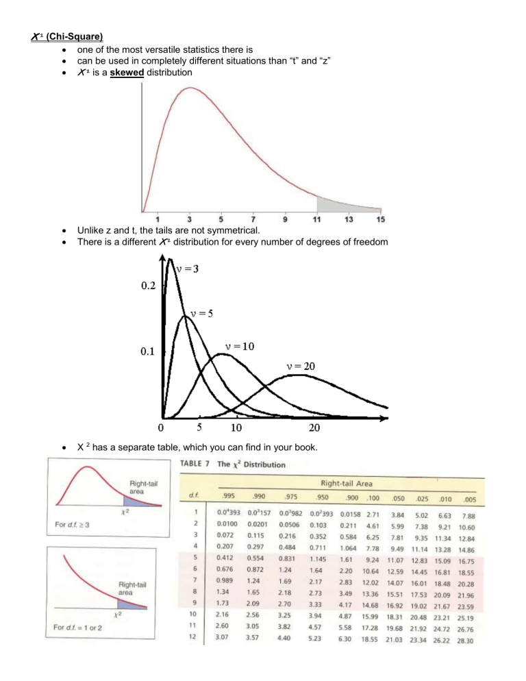
X 2 (Chi-Square)

one of the most versatile statistics there is

can be used in completely different situations tha n “t” and “z”
 X 2 is a skewed distribution

Unlike z and t, the tails are not symmetrical.

There is a different X 2 distribution for every number of degrees of freedom

X 2 has a separate table, which you can find in your book.


X 2 can be used for many different kinds of tests.

We will learn 3 separate kinds of X 2 tests.
Matrix Chi-Square Test
(a.k.a. “Independence” Test)

Compares two qualitative variables.

QUESTION: Does the distribution of one variable change from one value to the other variable to another.
EXAMPLES

Are the colors of M&Ms different in big bags than in small bags?

In an election, did different ethnic groups vote differently?

Do different age groups of people access a website in different ways (desktop, laptop, smartphone, etc.)?
The information is generally arranged in a contingency table (matrix).

If you can arrange your data in a table, a matrix chi-square test will probably work.
For example:
Suppose in a TV class there were students at all 5 ILCC centers, in the following distribution:
Center
Algona
E’burg
E’ville
Spenc.
S.L.
Male
5
3
4
4
3
Female
7
2
4
7
3
Does the distribution of men and women vary significantly by center?

Our question essentially is —Is the distribution of the columns different from row to row in the table?

A significant result will mean things ARE different from row to row.

In this case it would mean the male/female distribution varies a lot from center to center.
The test process is still the same:
1. Look up a critical value.
2. Calculate a test statistic.
3. Compare, and make a decision.
Critical Value:

d.f. = (R – 1)(C – 1) one less than the number of rows
TIMES one less than the number of columns

Your calculator will give this correctly.
 Look up d.f. and α in the X 2 table.


Note that X 2 can have a wide range of values, depending on the degrees of freedom. The numbers are much more varied than “z” and “t”.
•
•
In this problem …
Since there’s no α given in the problem, let’s use α = .05
There are 5 rows and 2 columns, so we have (4)(1)=4 df
• X 2 (4,.05) = 9.49
Test Statistic

Most graphing calculators and spreadsheet programs include this test.

On a TI-83 or 84, this is the test called “X 2 Test” built into the “Tests” menu.
1. Enter the observed matrix as [A] in the MATRIX menu.

Press MATRX or 2 nd and x -1 , depending on which TI-83/84 you have.
 Choose “EDIT” (use arrow keys)

Choose matrix [A] (just press ENTER)

Type the number of rows and columns, pressing ENTER after each.

Enter each number, going across each row, and hitting ENTER after each.
2. Press 2 nd and MODE to QUIT back to a blank screen.

3. Go to STAT, then TESTS, and choose X 2 -Test (easiest with up arrow)
(Note on a TI84 this is “X 2 Test”, not “X 2 GOF Test”)
4. Make sure it says [A] and [B] as the observed and expected matrices. If it does just hit ENTER three times.
RESULT

.979 < 9.49

NOT significant
5. The read-out will give you X 2 and the degrees of freedom.

Categorical Chi-Square Test
(a.k.a. “Goodness of Fit” Test)
QUESTION:

Is the distribution of data into various categories different from what is expected?

Key idea —you have qualitative data (characteristics) that can be divided into more than 2 categories.
EXAMPLES
 ·Are the colors of M&Ms distributed as the company says?

Is the racial distribution of a community different than it used to be?

When you roll dice, are the numbers evenly distributed?
You’re comparing what the distribution in different categories should be with what it actually is in your sample.
HYPOTHESES:
H
1
: The distribution is significantly different from what is expected.
H
0
: The distribution is not significantly different from what is expected.
CRITICAL VALUE:

df = k – 1

one less than the number of categories

IMPORTANT: A TI-84 will not calculate this correctly.
TEST STATISTIC:

This test is on the TI-84, but not on the TI-83.

Unless you have a TI-84, you will need to use the formula.
If you have a TI84, here’s what you do …
Enter the numbers



Go to STAT  EDIT
Type the
Type the observed expected
values in L1.
values in L2. (You can just take each percent times the total.)
 2 nd / MODE (QUIT)
Do the test




EXAMPLE
Go to STAT  TESTS
Choose choice “D” (you may want to use the up arrow)… X 2 GOF-Test
Hit ENTER repeatedly. (It doesn’t actually matter what you put on the “
In the read-out what you care about is X 2 .
df ” line.)
You think your friend is cheating at cards, so you keep track of which suit all the cards that are played in a hand are. It turns out to be:
 ♦
 ♥
 ♣
 ♠




4
2
13
1

You’d normally expect that 25% of all cards would be of each suit. At the .01 level of significance, is this distribution significantly different than should be expected?
Critical Value

There are 4 categories, so we have 3 degrees of freedom.
 X 2 (3, .01) = 11.34
Test Statistic
STAT  EDIT
L1
4
L2
5
2
13
1
------
L2(5) =
5
5
5
------
L3
------
2 nd  MODE (QUIT)
STAT  TESTS  X 2 GOF-Test
X 2 GOF-Test
Observed:L1
Expected:L2
df:3
Calculate Draw
X 2 GOF-Test
X 2 =18
P=.001234098
CNTRB={.2 1.8 …
 X 2 = 18

(Unless you change the degrees of freedom, the p-value and d.f. numbers will be wrong, but X 2 should still be correct.)
RESULT:

18 > 11.34

Significant
If you don’t have access to a TI-84 (or other technology), the alternative is to use this formula …


O

E

2

2 
E
For each category:

Subtract observed value (what it is in your sample) minus expected value (what it should be).

Square the difference.

Divide the square by the expected value.
Add up the answers for all categories.
Example:
A teacher wants different types of work to count toward the final grade as follows:
Daily Work  25%
Tests
Project
Class Part.
 50%
 15%
 10%
When points for the term are figured, the actual number of points in each category is:
Daily Work  175
Tests
Project
Class Part.
 380
 100
 75
TOTAL POINTS = 730
Was the point distribution significantly different than the teacher said it would be? (Use α = .05)

CRITICAL VALUE
There are 4 categories, so there are 3 degrees of freedom.

X 2 (3,.05) = 7.81
This time it’s easiest to take each percent times the total for the expected values.
L1 L2
4
2
13
1
.25*730
.5*730
.15*730
.1*730
------ ------
L2(5) =
L3
------
L1
4
2
L2
182.5
365
13
1
109.5
73
------ ------
L2(5) =
L3
------
X 2 GOF-Test
X 2 =1.803652968
P=.6141403319
df=3
CNTRB={.308219…
RESULT
1.804 < 7.81, so NOT significant.
The division is roughly the same as what it was supposed to be.
Standard Deviation X 2 -Test
One use for X 2 is testing standard deviations.

This is most often used in quality control situations in industry.
QUESTION:

Is the standard deviation too large?

Is the data too spread out?
HYPOTHESES:
H
0
: The standard deviation is close to what it should be.
H
1
: The standard deviation is too big. (It is significantly larger than it should be.)
CRITICAL VALUE:

df = n – 1
 Look up α in the column at the top.
FORMULA:
2
( n

1 ) s
2
 
 2
Important —this test is NOT built into the TI-83. You MUST do it with the formula.
 σ is what the standard deviation should be.
 s is what the standard deviation actually is in your sample.

Example:
Bags of Fritos
®
are supposed to have an average weight of 5.75 ounces. An acceptable standard deviation is
.05 ounces.
Suppose a sample of 6 bags of Fritos
®
finds a standard deviation of .08 ounces. Is this unacceptably large?
(Use α = .05)

df = 6 – 1 = 5

Critical: X 2 = 11.07
Test: 5*.08
2 /.05
2 = 12.8
(Note that the mean is irrelevant in the problem.)

This is significant.
Example:
A wire manufacturer wants its finished product to be within a certain tolerance. For this to happen, the standard deviation should be less than 2.4 microns. Suppose a sample of size 20 finds the standard deviation is 3.1 microns. Do they need to adjust the machinery? Use α = .01
EXAMPLE:
When checking out, customers prefer consistent service —rather than lines that move at different speeds. A discount store company finds that in the past the average wait to check out has been 249 seconds, with a standard deviation of 46 seconds. They try a new check-out method at 12 different check lanes and find that the standard deviation with the new method is 54 seconds. Does this mean the new method has a significantly bigger variation in wait time? Do a standard deviation x 2 test at the 10% level of significance.
Statistical Process Control
In business, statistical tests are rarely performed in the way we do them in class.

It would be time-consuming and costly to calculate values of t, z, or X 2 each time we wanted to check the status of something.
Instead, in most business settings, a process called Statistical Process Control is used.

The methods were perfected by Iowan William Edwards Deming in the 1950s.

After World War II, the U.S. State Department sent Deming to Japan to assist Japanese industry in recovering after the war.

His methods were applied by companies like Mitsubishi, Honda, Toyota, Sanyo, and Sony —leading to the rise of Japanese industry in the world.

American and European companies started applying these m ethods in the 1980s and ‘90s.
In most cases, statistical process control involves keeping track of sample data over time on a control chart .

These use the idea that every process will vary to some extent.

The key is to see when it is out of control .

There are many types of control charts, but the majority are centered on the mean and marked off with standard deviations.

Control charts are often shaded to indicate the easiest method of interpretation:

Often the middle area (between -1 and 1 S.D.) is shaded green —meaning things are O.K. o There may be some variation, but it’s not enough to worry about.

The areas between 1 and 2 and -1 and -2 SD are often shaded yellow —meaning careful observation is necessary. o A potential problem may occur, but no adjustment is needed yet.

The areas beyond -2 and 2 are often shaded red —meaning the process is out of control and adjustments need to be made. o This is equivalent to a significant result on a statistical test.
There are other things that can indicate an out of control process as well:

The most common is a long run of data (10 – 12 in a row) on the same side of the mean.


Another is a short run of data (3 – 5 in a row) in the “yellow” zone.
Control charts can be used for

Quality control (in both manufacturing & services)

Correct allotment of materials

Efficient distribution of personnel

Efficient use of time on different projects

Recognizing any pattern that might indicate a problem

Recognizing superior performance of any sort (bei ng “out of control” in a positive way)
In addition to being marked off with standard deviations, sometimes control charts are marked off with the numbers that produce various results on a statistical test.
 In this case, the “green/yellow” boundary is often a result that would produce a result at the 10% level of significance.
 The “yellow/red” boundary is often a result that would produce a result at either the 5% or 1% level of significance.