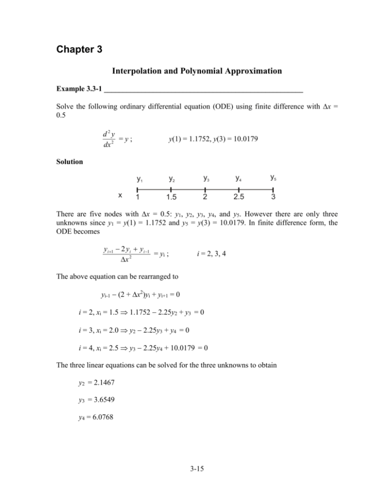
Chapter 3
Interpolation and Polynomial Approximation
Example 3.3-1 _____________________________________________________
Solve the following ordinary differential equation (ODE) using finite difference with x =
0.5
d2y
=y;
dx 2
y(1) = 1.1752, y(3) = 10.0179
Solution
x
y1
y2
y3
y4
y5
1
1.5
2
2.5
3
There are five nodes with x = 0.5: y1, y2, y3, y4, and y5. However there are only three
unknowns since y1 = y(1) = 1.1752 and y5 = y(3) = 10.0179. In finite difference form, the
ODE becomes
yi 1  2 yi  yi 1
= yi ;
x 2
i = 2, 3, 4
The above equation can be rearranged to
yi-1  (2 + x2)yi + yi+1 = 0
i = 2, xi = 1.5  1.1752  2.25y2 + y3 = 0
i = 3, xi = 2.0  y2  2.25y3 + y4 = 0
i = 4, xi = 2.5  y3  2.25y4 + 10.0179 = 0
The three linear equations can be solved for the three unknowns to obtain
y2 = 2.1467
y3 = 3.6549
y4 = 6.0768
3-15
Example 3.3-2 _____________________________________________________
Solve the following ordinary differential equation (ODE) using finite difference with x =
0.25
d2y
= 4y ;
dx 2
y(0) = 1,  4
dy
= y at x = 1.0
dx
Solution
x
y1
y2
y3
y4
y5
0
0.25
0.50
0.75
1.00
y6
There are five nodes with x = 0.25: y1, y2, y3, y4, and y5. The first node is given since y1 =
y(0) = 1. However there is one more extra node on the right y6 due to the derivative boundary
condition at x = 1.0. In finite difference form, the ODE becomes
yi 1  2 yi  yi 1
= 4yi ;
x 2
i = 2, 3, 4, 5
The above equation can be rearranged to
yi-1  (2 + 4x2)yi + yi+1 = 0
i = 2, x = 0.25  1.0  2.25y2 + y3 = 0
i = 3, x = 0.50  y2  2.25y3 + y4 = 0
i = 4, x = 0.75  y3  2.25y4 + y5 = 0
i = 5, x = 1.00  y4  2.25y5 + y6 = 0
y6 can be eliminated by using the boundary condition  4
4
dy
= y at x = 1.0
dx
y6  y4
= y5  y6 =  0.125y5 + y4
2  0.25
The equation at node 5 becomes
2y4  2.375y5 = 0
The four linear equations can be solved for the four unknowns to obtain
y2
0.6248
y3
0.4058
y4
0.2822
3-16
y5
0.2427
Example 3.3-3 _____________________________________________________
Solve the following ordinary differential equation (ODE) using finite difference with x =
0.25
dy
d2y
x
+ x2y = x3 ;
2
dx
dx
y+
dy
dy
= 1 at x = 0, y +
= 2 at x = 1
dx
dx
Solution
y0
x
y1
y2
y3
y4
y5
0
0.25
0.50
0.75
1.00
y6
There are five nodes with x = 0.25: y1, y2, y3, y4, and y5. However there are two more extra
nodes y0 and y6 due to the derivative boundary conditions. In finite difference form, the ODE
becomes
yi 1  2 yi  yi 1
y  yi 1
 xi i 1
+ xi2yi = xi3 ;
2
x
2x
i = 1, 2, 3, 4, 5
The above equation can be rearranged to
(2 + xi x)yi-1 + (2x2xi2  4)yi + (2  xi x)yi+1 = 2x2xi3
i = 1, xi = 0  2y0  4y1 + 2y2 = 0
y0 can be replaced with y1 and y2 from the boundary condition at x = 0.
y1 +
y2  y0
= 1  2y0 = y1 + 2y2  1   3y1 + 4y2 = 1
2 x
i = 2, 3, 4  (2 + xi x)yi-1 + (2x2xi2  4)yi + (2  xi x)yi+1 = 2x2xi3
i = 5, xi = 1.00  2.25y4  3.875y5 + 1.75y6 = 0.125
y6 can be replaced with y4 and y5 from the boundary condition at x = 1.
y5 +
y6  y4
= 2  y6 = y4  0.5y5 + 1
2 x
2.25y4  3.875y5 + 1.75(y4  0.5y5 + 1) = 0.125
The five linear equations can be solved for the five unknowns to obtain
y1
0.41371
y2
0.56028
y3
0.71506
3-17
y4
0.88689
y5
1.08896