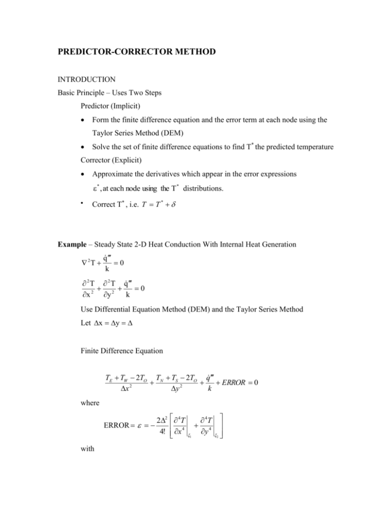
PREDICTOR-CORRECTOR METHOD
INTRODUCTION
Basic Principle – Uses Two Steps
Predictor (Implicit)

Form the finite difference equation and the error term at each node using the
Taylor Series Method (DEM)

Solve the set of finite difference equations to find T* the predicted temperature
Corrector (Explicit)

Approximate the derivatives which appear in the error expressions
 * , at each node using the T * distributions.

Correct T* , i.e. T  T *  
Example – Steady State 2-D Heat Conduction With Internal Heat Generation
 2T 
q 
0
k
 2 T  2 T q 


0
k
x 2 y 2
Use Differential Equation Method (DEM) and the Taylor Series Method
Let x  y  
Finite Difference Equation
TE  TW  2TO TN  TS  2TO q 


 ERROR  0
x 2
y 2
k
where
ERROR    
with
22   4T

4!  x 4


1
 4T
y 4


2 

x w  1  x E
yS   2  y N
Predictor step
For this step assume =0 and solve the set of finite difference equations to
obtain values of T * ' s. The equation solved for interior points is:
TE * TW * 4TO  TN * TS *  
*
q 2
k
Corrector step
Determine the approximation for
 4T
x 4
 4T
y 4
and
O
O
How do we find an approximation for the derivatives at O?
Use Taylor Series expansions.
How many expansions do we need?
Introduce weighting coefficients to find out.
What conditions do we use to evaluate the weighting coefficients?
For the grid shown, is any special treatment needed near the
boundaries?
Interior node

WW W
O
E
EE
Approximation for
 4T
x 4
O
Weighting
Coefficients
Taylor Series Expansions
T
x O

2  2 T
2 x 2 O

3  3 T
3! x 3 O

4  4 T

4! x 4 O
TEE  TO  2

( 2 ) 2
2!

( 2 ) 3
3!

( 2 ) 4
4!
[C]
TW  TO  

2
2!

3
3!

4
4!
[D]
TWW  TO  2

( 2 ) 2
2!

( 2 ) 2
3!

( 2 ) 4
4!
[A]
TE  TO  
[B]
After summing the above equations requirements on coefficients of derivatives
are:
T
[COEF] x
 0  A  2B  C  2D
O
A  2B  C  2D  0
[COEF]
 2T
2
(2) 2
2
(2) 2

0

A

B

C

D
2
2
2
2
x 2 O
A  4B  C  4D  0
[COEF]
 3T
3
(2) 3
3
(2) 3

0

A

B

C

D
3!
3!
3!
3!
x 3 O
A  8B  C  8D  0
[COEF]
 4T
4
( 2 ) 4
4
( 2 ) 4

1

A

B

C

D
4!
4!
4!
4!
x 4 O
A  16B  C  16D 
4!
4
Solution of this simultaneous set of equations is:
AC
4
1
, BD 4
4


Approximation becomes
TEE * 4TE * 6TO * 4TW * TWW *
 4T

 O(2 )
x 4 O
4
Error based upon predictor temperatures is:
*  

22 1
(TEE * 4TE * 6TO * 4TW * TWW * ) 
(4!) 4
(TSS * 4TS * 6TO * 4TN * TN * )

At near wall nodes

W
O
E
EE
EEE
 4T
What is the appropriate expression for
?
x 4 O
Weighting
Coefficients
[A]
Taylor Series Expansions
TW  TO  
T
2  2 T
3  3 T
4  4 T



x O 2! x 2 O 3! x 3 O 4! x 4 O
[B]
TE  TO  
[C]
TEE  TO  2
[D]
TEEE  TO  3

2
2!

( 2 ) 2
2
(3) 2

2
3
3!

( 2 ) 3
3!
(3) 3

3!

4
4!
( 2 ) 4
4!
(3) 4

4!


Requirements
T
[COEF] x
 0  A  B  2C  3D
O
 A  B  2C  3D  0
 2T
2
2
(2) 2
(3) 2

0

A

B

C

D
2!
2!
2!
2!
x 2 O
A  B  4C  9D  0
[COEF]
 3T
3
3
( 2 ) 3
(3) 3
[COEF] x 3  0  A 3!  B 3!  C 3!  D 3!
O
 A  B  8C  27D  0
 4T
4
4
(2) 4
(3) 4

1

A

B

C

D
4!
4!
4!
4!
x 4 O
4!
A  B  16C  81D  4

[COEF]
Simultaneous solution of the set of equations
A
1
,
4
B
6
4 ,
C
4
,
4
D
So
TW * 4TO * 6TE * 4TEE * TEEE *
 4T

 O()
x 4 O
4
The error term is:
1
4

22 1
*
*
*
*
*
 
(
T

4
T

6
T

4
T

T
)
W
O
E
EE
EEE
(4!) 4
*
(TSS * 4TS * 6TO * 4TN * TN * )

To generate the corrected solution, we now introduce the error terms into the
equation and solve.
TE TW 4TO  TN TS
q 2

*
4
4k
Here we are solving a linear system with the same coefficient matrix used for the
predictor step, but with a modified right hand side. With the right choice of
solution method (e.g. LU decomposition), this can be substantially less time
consuming than the original predictor solution. If A is the coefficient matrix then
the correction equation can be written as:
 
 

T  T *    T *  A1 *
Here I've added arrows over symbols to emphasize that we are dealing with the
vectors of all mesh point temperatures and vector of all mesh point errors.