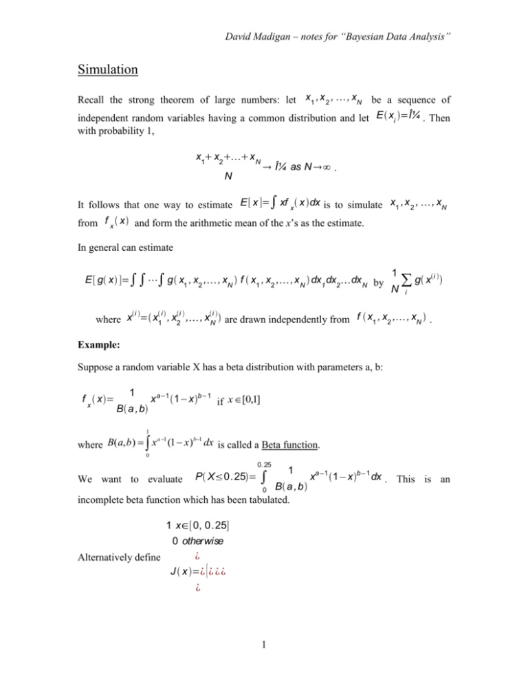
David Madigan – notes for “Bayesian Data Analysis”
Simulation
Recall the strong theorem of large numbers: let x1 ,x 2 ,
, xN be a sequence of
independent random variables having a common distribution and let E xi
with probability 1,
x1 x2
xN
μ as N
μ . Then
.
N
xf x x dx is to simulate x1 ,x 2 ,
It follows that one way to estimate E x
from f x x and form the arithmetic mean of the x’s as the estimate.
, xN
In general can estimate
E g x
g x1 , x2 ,
i
where x
x1i , x2i ,
, xN f x1 , x2 ,
,x N dx1 dx2
dx N by
1
N
, x Ni are drawn independently from f x1 , x2 ,
g xi
i
, xN .
Example:
Suppose a random variable X has a beta distribution with parameters a, b:
f
x
x
1
xa
1
1 x
B a ,b
b 1
if x [0,1]
1
a 1
b 1
where B( a, b )   x (1  x ) dx is called a Beta function.
0
0.25
We want to evaluate
P X 0.25
1
B a ,b
incomplete beta function which has been tabulated.
0
1x
0, 0.25
0 otherwise
Alternatively define
J x
1
xa
1
1 x
b 1
dx . This is an
David Madigan – notes for “Bayesian Data Analysis”
1
Then P X 0.25
E J x
J x f x x dx
0
So
P X 0. 25
estimate
1
N
J x by
i
simulating
x1 ,x 2 ,
, xN from
1
J x . 
i
N
This general procedure is called Monte Carlo Integration.
x1 ,x 2 ,
, xN and letting P X 0. 25
How do you draw random variables from f x x ?


Underlying many of the methods we will discuss for simulation will be the
requirement to generate random number e.g. a random number between 0 and 1.
Random number generation and assessing random number generators is a major
industry in itself. We will just assume that we have some method for doing it.
e.g. X n
1
Xn
aXn c mod m then
m
is approximately U 0, 1 .
Note the examples in the book
– generating a random permutation
estimating the number of distinct entries in a large set
Simulating continuous random variables
The Inverse Transformation Method
(method 1)
Proposition:
Consider a random variable x1 , x 2 , , xN with CDF F X x . Define a new random
variable Y F X x . Then Y ~ unif 0, 1 .
Proof:
FY y
P Y y
P FX x
y
1
P X FX y
F X F X1 y
sin ce F X is monotone

y so Y unif 0,1

Corollary:
2
David Madigan – notes for “Bayesian Data Analysis”
Let U unif 0, 1 . Define a random variable X F
the CDF of X.
1
U
where F is a CDF. Then F is
Proof:
FX x
P X x
P F
1
u
x
P u F x
F x .

Thus, if we know how to invert F X , we can simulate X by generating a random u ~ U(0,
1
1) and letting X F
u .
Example:
Simulating a Weibull. For a Weibull random variable X have:
x
FX x
Then F
1
α
β
1 e
u is that value of X such that:
x
α
β
1 e
x
e
x
u
α
β
1 u
α
log 1 u
β
1
x β
log 1 u α
X generated in this fashion will have Weibull α , β
distribution.
Note:
This method only works when F X is invertible which will not often be the case.
The rejection method
(method 2)
Suppose there is a density g x which is “close” to the density f that we wish to
simulate from but it is much easier to simulate from g than f (e.g. f might be
gamma and g Weibull). Then provided c such that
f x
g x
c for all x, we can use g to get simulations from f .
3
David Madigan – notes for “Bayesian Data Analysis”
Note:
g x
must have support at least as big as f x .
Here is how it works:
Step 1 Simulate Y having density g and simulate a random number U.
Step 2
f Y
If U
set X Y . Otherwise return to step 1.
cg Y
Claim: that the value X has density function f .
Proof:
P X x
P Y
P Y x
u
N
x
PY x u
f Y
cg Y
f Y
P Y x
f Y
u
P u
f Y
P u
cg Y
x
f y
Y y g y dy
cg Y
cg Y
f Y
cg Y
x
g y dy
f y dy
cg y
P u
f Y
cP u
f Y
cg Y
cg Y
The denominator does not involve x.
f Y
cP u
But lim P X x 1
cg Y
x
1
4
Pu
f Y
1
cg Y
c
.
David Madigan – notes for “Bayesian Data Analysis”
Note:
Since P u
f Y
1
cg Y
c
, the number of iterations until an acceptance will be geometric
with mean c. Thus it is important to choose g (Y ) so that c is small.
Note:
However, a difficulty with the rejection method is that in many applications, c is hard to
compute. Often end up choosing c very conservatively large thereby resulting in very
high computational costs.
Sampling Importance Resampling
(method 3) (Rubin, 1987)
Again, assume there is a density g x which is close to the density f that we want to
simulate from. Then to generate a sample of size n from f, proceed as follows:
1. draw x1 ,x 2 ,
, xN from g x
2. sample a value x from the set
x1 , x2 ,
each xi is proportional to w x
, xN
where the probability of sampling
f x
g x
3. sample a second value x using the same procedure, but excluding the already
sampled value from the set
4. repeatedly sample without replacement n – 2 more times.
“Proof”:
Each of the n x’s is drawn with possibility:
g x
g x
w x
w x dx
as
N
n
f x
f x

f x dx
5
David Madigan – notes for “Bayesian Data Analysis”
Note:
SIR is subject to the same problems as rejection sampling but has the advantage that it
converges provided w x
without explicitly requiring max w x .
Example: (beta distribution)
Suppose want to simulate from f x x
1
xa
1
1 x
B a ,b
our candidate (also called the “envelope” distribution) g x
Then
d
f
is bounded iff α , β
g
xa
1
b 1
1 x
xa
2
b 1
, x [0,1] . We chose as
1 , x [0,1] .
1
1 x
b 2
x b 1
1 x a 1 so max at 0 or 1 or
dx
1 a
1 b
Use either rejection sampling or SIR.
xα
If α 0, β 1 then use g x Î ±
Î x
±Î±
Can simulate from g x
1
1
by the inverse transformation method:
1
x
α 1
g x
Î ±
t
α
dt x
u
x u
α
0
1
So if u unif 0,1 , x u
α
α 1
Î ±
x
Methods for simulating Normal Random Variables
1. Sum of 12 uniforms (approximate algorithm)
12
X
u
i
6 ,
i 1
ui unif 0, 1
12
E X
E u
i
i 1
6 12
1
6 0
2
6
David Madigan – notes for “Bayesian Data Analysis”
12
V X
V u
12
i
1
1
2
i 1
and X is approximately normal by Central Limit Theorem. This is a fairly crude
approximation but may be adequate for some applications.
2. Rejection Sampling
2
First note that if f Z z
Then letting x
z
1
2
e
(i.e. Z ~ N(0, 1))
2Ï€
z
2
2
fX x
( FX x
P X x
P
x
Try candidate distribution gX x
e
2
Then
1
( e
2
f x
2
g x
2Ï€
e
x
, 0 x
x
e
2
FZ
2
1 since if e
x' 1
2
x
fX x
fZ x
x
x
2
2
1
2e
2
e
Ï€
2
1
1
x' 1
2
2
1
e
2
x 1
2
2e
Ï€
1.3155
0 which is impossible )
So, the procedure is:
1. generate a realization from gX x
e
x
(Inverse transform)
2. generate u unif 0, 1
1
x 1
fZ x )
(i.e. exp(1))
2Ï€
1
x 1
FZ x
1
2
2
2
e
2Ï€
x z
x
x
2
3. if u e 2
then accept x. Else go to 1.
4. generate u unif 0, 1 . If u unif 0, 1 .
Note:
This is quite efficient requiring an average of 1.32 iterations per acceptance.
3. Box-Muller
Let X, Y ~ N(0, 1), X, Y independent
Consider a transformation to polar coordinates:
7
David Madigan – notes for “Bayesian Data Analysis”
R2 X 2 Y2
Y
θ tan 1
X
To get the joint distribution of R 2 and  need Jacobian of the transformation
J
d
d
x
y
θ
θ
x
y
2x
1
1
y2
x
2y
y
1
x2
y2 1
x
2
f
2
R , θ
d , θ
2
So R and θ
z
1
Since f X , Y x , y
1
2
2
2
x
2
y
2
e
2Ï€
1
2Ï€
d
e
2
1
1
2
2
d
e
2
1
for 0 d
2Ï€
2
are independent. Furthermore R exp
2
So proceed by generating R and θ
1
and 0 θ
, θ
2
Simulating a beta random variable
fX x
Γ n m
unif 0, 2Ï€ .
and then setting X Rcosθ , Y Rsinθ
resulting in two independent standard normal random variables.
X B n, m
2Ï€
x
n 1
1 x
m 1
, 0 x 1
Γ n Γ m
Consider the n-th smallest of n + m – 1 random 0-1 numbers.
8
David Madigan – notes for “Bayesian Data Analysis”
U n
x
fU
n
x
P U
x
x n 1 1 x m 1 arrangements
arrangements ways to pick x
n m 1
n 1
fu x P U x
m 1
arrangements
ways of splitting around x
n m 2
n m 1 !
n 1
n 1 ! m 1 !
U (n) has a beta distribution with params n of m.
A problem with this approach is that finding the n-th smallest of n + m – 1 random
numbers is expensive if n, m are large.
9