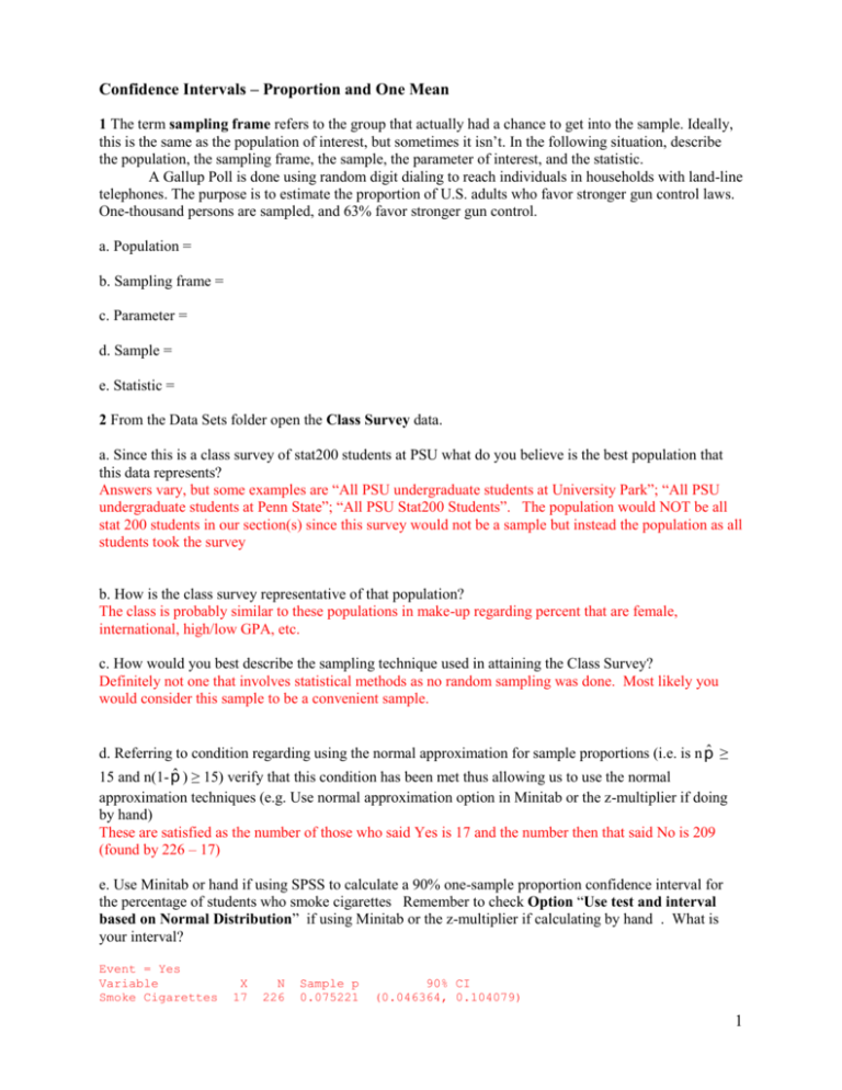
Confidence Intervals – Proportion and One Mean
1 The term sampling frame refers to the group that actually had a chance to get into the sample. Ideally,
this is the same as the population of interest, but sometimes it isn’t. In the following situation, describe
the population, the sampling frame, the sample, the parameter of interest, and the statistic.
A Gallup Poll is done using random digit dialing to reach individuals in households with land-line
telephones. The purpose is to estimate the proportion of U.S. adults who favor stronger gun control laws.
One-thousand persons are sampled, and 63% favor stronger gun control.
a. Population =
b. Sampling frame =
c. Parameter =
d. Sample =
e. Statistic =
2 From the Data Sets folder open the Class Survey data.
a. Since this is a class survey of stat200 students at PSU what do you believe is the best population that
this data represents?
Answers vary, but some examples are “All PSU undergraduate students at University Park”; “All PSU
undergraduate students at Penn State”; “All PSU Stat200 Students”. The population would NOT be all
stat 200 students in our section(s) since this survey would not be a sample but instead the population as all
students took the survey
b. How is the class survey representative of that population?
The class is probably similar to these populations in make-up regarding percent that are female,
international, high/low GPA, etc.
c. How would you best describe the sampling technique used in attaining the Class Survey?
Definitely not one that involves statistical methods as no random sampling was done. Most likely you
would consider this sample to be a convenient sample.
d. Referring to condition regarding using the normal approximation for sample proportions (i.e. is n p̂ ≥
15 and n(1- p̂ ) ≥ 15) verify that this condition has been met thus allowing us to use the normal
approximation techniques (e.g. Use normal approximation option in Minitab or the z-multiplier if doing
by hand)
These are satisfied as the number of those who said Yes is 17 and the number then that said No is 209
(found by 226 – 17)
e. Use Minitab or hand if using SPSS to calculate a 90% one-sample proportion confidence interval for
the percentage of students who smoke cigarettes Remember to check Option “Use test and interval
based on Normal Distribution” if using Minitab or the z-multiplier if calculating by hand . What is
your interval?
Event = Yes
Variable
Smoke Cigarettes
X
17
N
226
Sample p
0.075221
90% CI
(0.046364, 0.104079)
1
f. For the interval, answer the following (if you values differ but are close – first decimal is correct – then
difference is probably due to rounding):
What is the sample proportion, p̂ ? .07
What is the z multiplier used for your interval? 1.65
What is the standard error? .017
What is the margin of error? 1.65*0.017 = 0.028
f. If the confidence level in part g were changed to 95% would your resulting interval be wider or
narrower? The interval would get wider since you increased your confidence from 90 to 95%.
Remember, the greater the confidence level the more “confident” you become that the interval contains
the true parameter value. A wider interval would increase your confidence since a wider interval would
give more possible outcomes. Mathematically this is also true because you will notice that at the
confidence level gets larger so does the multiplier.
g. The U.S. Government reported that 23% of US adults age 18-24 smoked cigarettes. Based on your
confidence interval do believe that this percentage is reasonable, too high, or too low for Penn State
students and explain why.
Since our interval does not contain 0.23 (i.e. 23%) and is less than this value we would conclude that the
governments reported value is too high for the PSU population.
3 For mean confidence intervals we call into use T-Table which can be found in this week’s folder. The
first concept to understand is the idea of Degrees of Freedom (DF). For our activity today, since we are
only concerned with one mean (either from one sample of a difference between paired data), DF = sample
size – 1 (i.e. n – 1). When finding confidence intervals, T-Table provides the t multiplier (t*) for the
confidence interval expression:
x  t* *
s
n if data is consists of only one sample
NOTE: you will notice that the DF column in this tables only increases by 1 from 1 to 30. After that
the increments vary. If your DF is NOT found in the table then conservatively use the CLOSEST
df in the table that does not exceed the DF of interest. For example, if the degrees of freedom were
37 then from the table use 30.
Find t-multipliers and DF from Table A2 for the following conditions:
Confidence Level 90%, n = 25: t* = 1.71
DF = 24
Confidence Level 95%, n = 25: t* = 2.06
DF = 24
Confidence Level 95%, n = 35: t* = 2.04
DF = 34
Confidence Level 99%, n = 35: t* = 2.75
DF = 34
2
What do you notice that happens to t* as the level of confidence increases for the same sample size?
The multiplier, t*, increases as the level of confidence increases
What do you notice that happens to t* as sample size increases for the same level of confidence?
The multiplier, t*, decreases as sample size increases
4 Using the Class Survey data, PSU wants to estimate the true SATM scores for its undergraduate
population. Assuming that our survey represents this population, calculate a 1-mean 95% confidence
interval to estimate the parameter. First we will do by hand and then using software. To start, the sample
mean ( x ) is 599 and n = 216 and s = 85.34.
a. Calculate the standard error of the mean.
s
n = 85.34/√216 = 5.81
b. What are the DF and t* from T-table?
DF = 215
t* = 1.98
c. Calculate the 95% Confidence Interval and provide an interpretation of this interval.
x  t* *
s
n = 599 ± 1.98*5.81 = 599 ± 11.504 = 587.496 ≤ u ≤ 610.504
d. Now use software to verify your results by calculating a 95% one-sample T confidence interval. Copy
and paste your output results below. Do your results by hand and those from software roughly match?
One-Sample T: SATM
Variable N Mean StDev SE Mean
95% CI
SATM 216 599.005 85.335 5.806 (587.560, 610.449)
The intervals by hand and software are comparable.
e. Write a sentence that explains what this interval means. We are 95% confident that the true mean
SATM score for the incoming freshman class at Penn State was between 587.56 and 610.449.
f. Based on the interval calculated, if Penn State claimed that the true mean SATM score for the 2005
incoming freshman was 610 would you believe them? Explain. Yes, since the score of 610 is in the
interval.
3