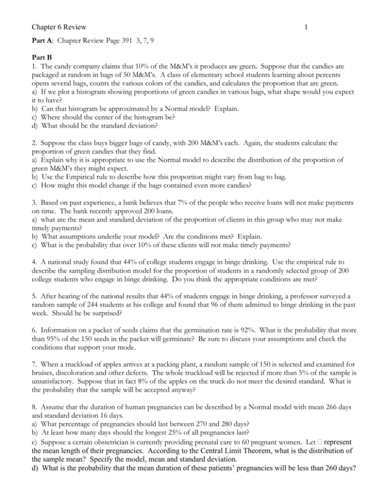
Chapter 6 Review
1
Part A: Chapter Review Page 391 3, 7, 9
Part B
1. The candy company claims that 10% of the M&M’s it produces are green. Suppose that the candies are
packaged at random in bags of 50 M&M’s. A class of elementary school students learning about percents
opens several bags, counts the various colors of the candies, and calculates the proportion that are green.
a) If we plot a histogram showing proportions of green candies in various bags, what shape would you expect
it to have?
b) Can that histogram be approximated by a Normal model? Explain.
c) Where should the center of the histogram be?
d) What should be the standard deviation?
2. Suppose the class buys bigger bags of candy, with 200 M&M’s each. Again, the students calculate the
proportion of green candies that they find.
a) Explain why it is appropriate to use the Normal model to describe the distribution of the proportion of
green M&M’s they might expect.
b) Use the Empirical rule to describe how this proportion might vary from bag to bag.
c) How might this model change if the bags contained even more candies?
3. Based on past experience, a bank believes that 7% of the people who receive loans will not make payments
on time. The bank recently approved 200 loans.
a) what are the mean and standard deviation of the proportion of clients in this group who may not make
timely payments?
b) What assumptions underlie your model? Are the conditions met? Explain.
c) What is the probability that over 10% of these clients will not make timely payments?
4. A national study found that 44% of college students engage in binge drinking. Use the empirical rule to
describe the sampling distribution model for the proportion of students in a randomly selected group of 200
college students who engage in binge drinking. Do you think the appropriate conditions are met?
5. After hearing of the national results that 44% of students engage in binge drinking, a professor surveyed a
random sample of 244 students at his college and found that 96 of them admitted to binge drinking in the past
week. Should he be surprised?
6. Information on a packet of seeds claims that the germination rate is 92%. What is the probability that more
than 95% of the 150 seeds in the packet will germinate? Be sure to discuss your assumptions and check the
conditions that support your mode.
7. When a truckload of apples arrives at a packing plant, a random sample of 150 is selected and examined for
bruises, discoloration and other defects. The whole truckload will be rejected if more than 5% of the sample is
unsatisfactory. Suppose that in fact 8% of the apples on the truck do not meet the desired standard. What is
the probability that the sample will be accepted anyway?
8. Assume that the duration of human pregnancies can be described by a Normal model with mean 266 days
and standard deviation 16 days.
a) What percentage of pregnancies should last between 270 and 280 days?
b) At least how many days should the longest 25% of all pregnancies last?
c) Suppose a certain obstetrician is currently providing prenatal care to 60 pregnant women. Let  represent
the mean length of their pregnancies. According to the Central Limit Theorem, what is the distribution of
the sample mean? Specify the model, mean and standard deviation.
d) What is the probability that the mean duration of these patients’ pregnancies will be less than 260 days?
Chapter 6 Review
9. The College Board reported the score distribution shown in the table
for all students who took the 2005 AP statistics exam.
a) Find the mean and standard deviation of the scores.
b) If we selected a random sample of 40 AP Statistics students, would
you expect their scores to follow a Normal model? Explain.
c) Consider the mean scores of random samples of 40 AP statistics
students. Describe the sampling model for these means (shape, center,
spread).
2
Score
5
4
3
2
1
% of Students
12.5
22.5
24.8
19.8
20.4
10. Carbon monoxide emissions for a certain kind of car vary with mean 2.9 g/mi and standard deviation
0.4g/mi. A company has 80 of these cars in its fleet. Let  represent the mean CO level for the company’s
fleet.
a) What is the approximate model for the distribution of ? Explain.
b) Estimate the probability that  is between 3.0 and 3.1 g/mi.
c) There is only a 5% chance that the fleet’s mean CO level is greater than what value?
11. A waiter named Bernard believes the distribution of his tips has a model that is slightly skewed to the right,
with the mean of $9.60 and a standard deviation of $5.40.
a) Explain why you cannot determine the probability that a given party will tip him at least $20.
b) Can you estimate the probability that the next 4 parties will tip an average of at least $15? Explain.
c) Is it likely that his 10 parties today will tip and average of at least $15? Explain.
12. Bernard the waiter usually waits on about 40 parties over a weekend of work.
a) Estimate the probability that he will earn at least $500 in tips.
b) How much does he earn on the best 10% of such weekends?
13. Suppose that the IQs of East State University’s students can be described by a Normal model with mean
130 and standard deviation 8 points. Also suppose that the IQs of students from West State University can be
described by a Normal model with mean 120 and standard deviation 10.
a) We select 1 student at random from East State. Find the probability that this student’s IQ is at least 125
points.
b) We select 1 student at random from each school. Find the probability that the East State student’s IQ is at
least 5 points higher than the West State student’s IQ.
c) We select 3 West State students at random. Find the probability that this group’s average IQ is at least 125
points.
d) We also select 3 East State students at random. What is the probability that their average IQ is at least 5
points higher than the average for the 3 West Staters?
Answers:
Part A: Back of the book
Part B:
1.
2. a) np = 20; nq = 180, both greater than 10.
b) About 68% will be between 7.9% and 12.1%. About 95% will be between 5.8% and 14.2% and about
99.7% should be between 3.7% and 16.3%
c) Sam center, less spread.
Chapter 6 Review
3
3. a) μ = 7% σ = 1.8%
b) Assume that clients pay independently of each other, that we have a random sample of all possible. np
= 14, nq = 186.
c) 0.048
4. a) About 68% will be between .405 and .475 About 95% will be between .370 and .510, and about
99.7% should be between .335 and .545. Conditions are met; it’s a random sample with np = 88 and
nq = 112.
5.
6.
7.
8.
9.
Probably not (reasoning)
0.081. Assume the seeds are a random sample and germinate independently.
0.088 using N(0.08, 0.022)
a) 21.1% b) 276.8 days or more
c) N(266, 2.07)
d) 0.002
a) μ = 2.869 σ = 1.312
b) No. The score distribution should resemble that in the population, somewhat uniform for scores 105
and about half as many 5s.

1.312 
c) Approximately N  2.869,

40 

10. a) N(2.9, 0.045)
b) 0.0131
c) 2.97 gm/mi
11. a) Can’t use a Normal model because the distribution is skewed.
b) 4 is probably not a large enough sample to say the average follows the Normal model.
c) No. This is 3.16 SDs above the mean.
12. a) 0.0003. model is N(384, 34.15)
b) $427.77 or more
13. a) 0.734
b) 0.653, N (10, 12.81)
c) 0.193, N(120, 5.774)
d) 0.751 N(10, 7.394)