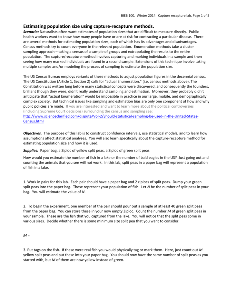
BIEB 100. Winter 2014. Capture recapture lab. Page 1 of 5
Estimating population size using capture-recapture methods.
Scenario: Naturalists often want estimates of population sizes that are difficult to measure directly. Public
health workers want to know how many people have or are at risk for contracting a particular disease. There
are several methods for estimating population sizes, each of which has its advantages and disadvantages.
Census methods try to count everyone in the relevant population. Enumeration methods take a cluster
sampling approach – taking a census of a sample of groups and extrapolating the results to the entire
population. The capture/recapture method involves capturing and marking individuals in a sample and then
seeing how many marked individuals are found in a second sample. Extensions of this technique involve taking
multiple samples and/or modeling the process of sampling to estimate the population size.
The US Census Bureau employs variants of these methods to adjust population figures in the decennial census.
The US Constitution (Article 1, Section 2) calls for "actual Enumeration.” (i.e. census methods above). The
Constitution was written long before many statistical concepts were discovered, and consequently the founders,
brilliant though they were, didn't really understand sampling and estimation. Moreover, they probably didn't
anticipate that "actual Enumeration" would be impossible in practice in our large, mobile, and demographically
complex society. But technical issues like sampling and estimation bias are only one component of how and why
public policies are made. If you are interested and want to learn more about the political controversies
(including Supreme Court decisions) surrounding the census and sampling see:
http://www.scienceclarified.com/dispute/Vol-2/Should-statistical-sampling-be-used-in-the-United-StatesCensus.html
Objectives. The purpose of this lab is to construct confidence intervals, use statistical models, and to learn how
assumptions affect statistical analyses. You will also learn specifically about the capture-recapture method for
estimating population size and how it is used.
Supplies: Paper bag, a Ziploc of yellow split peas, a Ziploc of green split peas
How would you estimate the number of fish in a lake or the number of bald eagles in the US? Just going out and
counting the animals that you see will not work. In this lab, split peas in a paper bag will represent a population
of fish in a lake.
1. Work in pairs for this lab. Each pair should have a paper bag and 2 ziplocs of split peas. Dump your green
split peas into the paper bag. These represent your population of fish. Let N be the number of split peas in your
bag. You will estimate the value of N.
2. To begin the experiment, one member of the pair should pour out a sample of at least 40 green split peas
from the paper bag. You can store these in your now empty Ziploc. Count the number M of green split peas in
your sample. These are the fish that you captured from the lake. You will notice that the split peas come in
various sizes. Decide whether there is some minimum size split pea that you want to consider.
M=
3. Put tags on the fish. If these were real fish you would physically tag or mark them. Here, just count out M
yellow split peas and put these into your paper bag. You should now have the same number of split peas as you
started with, but M of them are now yellow instead of green.
BIEB 100. Winter 2014. Capture recapture lab. Page 2 of 5
4. Shake the paper bag for a while to mix the green and yellow split peas (the fish are swimming around!).
5. Fish in your lake again. Take out a random sample of split peas from your paper bag. This time make it
around 60 split peas. Let n be the sample size. Count the number of yellow (tagged) split peas and call it T.
6. What fraction of split peas in the second sample are yellow? Use this fraction to estimate N, the total number
of split peas in the bag. Write down an equation for N and solve it using your data.
N=
7. Describe your sampling data in a 2x2 table (note that you won't be able to fill in all these cells just with your
actual counts. Some of the cells you will only be able to fill in once you have estimated the population size).
In first sample
(meaning they
were tagged)
Not in first sample
(meaning they
weren't tagged)
Total
In second
sample
Not in second
sample
Total
8. Your solution for N only makes sense as an estimate of the population size if it is reasonable that the sample
percentage of yellow split peas (tagged fish) would be an unbiased estimate of the population percentage of
yellow split peas (tagged fish). This depends on many assumptions. As a section, identify some of these
assumptions and discuss how each would affect the resulting estimate of N. It may be easier to identify
assumptions if you think about the process of tagging fish in the real world. Do any of these assumptions also
affect your split pea model system? If they do, how could you modify your split pea model to be more realistic?
BIEB 100. Winter 2014. Capture recapture lab. Page 3 of 5
9. It turns out that the straightforward formula for estimating population size:
size of population = # tagged in population ´
size of 2nd sample
# tagged in 2nd sample
(equation 1)
tends to overestimate the true population size. An unbiased estimator is:
size of population = ( # tagged in population +1) ´
(size of 2nd sample +1)
( # tagged in 2nd sample +1)
-1
(equation 2)
(link to original reference for this estimator).
Use equation 2 below when you use your confidence intervals for the population proportion of tagged fish to
construct confidence intervals for the population size.
10. You now have taken a sample from your population. Use it to construct a confidence interval for population
size by two different methods.
11. First, make a bootstrap confidence interval. Use the StatKey applet here:
http://www.lock5stat.com/statkey/bootstrap_1_cat/bootstrap_1_cat.html
Click Edit Data and put in the counts from your sample (T and n). Generate a bootstrap distribution based on this
sample data. If you click Two-Tail then the tails of the distribution will be shaded in red. By default the applet
starts with 95% of the dots black. What is your 95% confidence interval? [Fill in the appropriate spaces in the
table below]
If you click on 0.950 you can change the confidence level (fraction of black dots in the middle). Change it to 0.80
corresponding to an 80% confidence interval. What is this?
How about a 60% confidence interval?
Confidence
level
Bootstrap
lower
bound for

Bootstrap
upper
bound for

Bootstrap
SE
Best
estimate
for N (pop.
size)
Bootstrap
lower
bound for
N
Bootstrap
upper
bound for
N
95%
80%
60%
12. If your sample size is large enough (T>10 and (n-T)>10) then you can make a confidence interval using the
normal approximation:
BIEB 100. Winter 2014. Capture recapture lab. Page 4 of 5
⌢ ⌢
⌢ *
p(1- p)
⌢
⌢
p ± z SE p where SE p =
n
z* comes from the normal distribution. For a 95% confidence interval, z* is 1.96. This means that 95% of the
points in a normal distribution are within 1.96 standard deviations of the mean. So 5% of the points have
standardized statistics that are more extreme (in absolute value) than 1.96.
You can find z* from the "Cumulative table" here: https://en.wikipedia.org/wiki/Standard_normal_table
The entry in the table corresponds to the probability that a statistic is less than Z (see as an example the yellow
area in the graph shown on the right of the table in the Wikipedia page. Z is the number in the left-most column
plus the number in the top row. So if you find 1.9 on the right, and 0.06 on the top, you will see 0.9750 in the
table. Make sure this makes sense that this would give you the z* to use for a 95% confidence interval. Figure
out what the appropriate z* should be for 80% and 60% and complete the table below.
Confidence
level
z*
95%
1.96
Normal SE
Normal
lower bound
for 
Normal
upper bound
for 
Normal
lower bound
for N
Normal
upper bound
for N
80%
60%
13. A 60% confidence interval is an interval constructed with a method that will cover the true population mean
60% of the time. This means that ~40% of your lab will have constructed 60% confidence intervals from their
samples that do not cover the true parameter – either or N. Count your peas to figure out your population
size. Did your intervals cover it? What fraction of your section had intervals that covered their true population
size?
60%
80%
95%
Fraction with confidence
intervals covering the true
N
14. In question 8 you listed some assumptions behind modeling the capture-recapture method for estimating
population size using split peas. Pick one of these assumptions and think carefully about what effect it would
have on your confidence interval if your assumption were wrong. Explain below.
BIEB 100. Winter 2014. Capture recapture lab. Page 5 of 5
The section below is included for students who are interested in seeing how statistical methods for estimating
population size play out in a public health context. There aren’t any questions to turn in, it’s just here to show
a rather important application of capture-recapture population size estimation.
Estimating population sizes is a crucial issue for health ministries and other public health organizations and can
be extraordinarily difficult when the at-risk populations are heavily stigmatized and difficult to find. A report
from the UNAIDS/WHO working group on HIV surveillance discusses advantages and disadvantages of several
methods of estimating the number of individuals at risk for HIV.
Be aware that this report talks quite frankly about several of the subpopulations at highest risk for HIV infection.
The report is called: Estimating the size of populations at risk for HIV. Issues and methods and can be
downloaded from here:
http://labs.biology.ucsd.edu/rifkin/courses/bieb100/w14/LabActivities/UNAIDS_estimatingpopsizes_en.pdf
You may find sections 3,4, and 5 most relevant. Section 4 has descriptions and examples of the methods.
Although there are some technical details in there that are beyond the scope of this course, you should be able
to get a sense for the methods. The last two methods in section 4 mention a Poisson distribution. A Poisson
distribution is a discrete probability distribution of the
number of events that happen in some unit interval of
time. These events are assumed to happen
independently of each other. Like other probability
distributions, it has a mean and variance – although it is
unusual in that its mean and variance are the same.
The shape of the distribution depends upon the mean.
At the right is a plot of Poisson distributions with
different means. That is, they have different mean
number of events in a unit interval of time. Here  is the
mean number of events per unit interval of time and k
is the actual outcome. The y axis tells you the
probability of getting k events in a given unit interval of
time.
(source: http://en.wikipedia.org/wiki/Poisson_distribution).