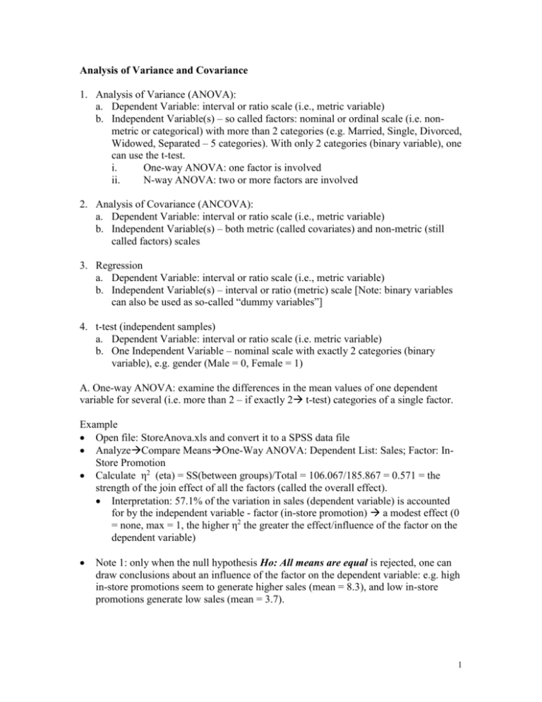
Analysis of Variance and Covariance
1. Analysis of Variance (ANOVA):
a. Dependent Variable: interval or ratio scale (i.e., metric variable)
b. Independent Variable(s) – so called factors: nominal or ordinal scale (i.e. nonmetric or categorical) with more than 2 categories (e.g. Married, Single, Divorced,
Widowed, Separated – 5 categories). With only 2 categories (binary variable), one
can use the t-test.
i.
One-way ANOVA: one factor is involved
ii.
N-way ANOVA: two or more factors are involved
2. Analysis of Covariance (ANCOVA):
a. Dependent Variable: interval or ratio scale (i.e., metric variable)
b. Independent Variable(s) – both metric (called covariates) and non-metric (still
called factors) scales
3. Regression
a. Dependent Variable: interval or ratio scale (i.e., metric variable)
b. Independent Variable(s) – interval or ratio (metric) scale [Note: binary variables
can also be used as so-called “dummy variables”]
4. t-test (independent samples)
a. Dependent Variable: interval or ratio scale (i.e. metric variable)
b. One Independent Variable – nominal scale with exactly 2 categories (binary
variable), e.g. gender (Male = 0, Female = 1)
A. One-way ANOVA: examine the differences in the mean values of one dependent
variable for several (i.e. more than 2 – if exactly 2 t-test) categories of a single factor.
Example
 Open file: StoreAnova.xls and convert it to a SPSS data file
 AnalyzeCompare MeansOne-Way ANOVA: Dependent List: Sales; Factor: InStore Promotion
 Calculate η2 (eta) = SS(between groups)/Total = 106.067/185.867 = 0.571 = the
strength of the join effect of all the factors (called the overall effect).
 Interpretation: 57.1% of the variation in sales (dependent variable) is accounted
for by the independent variable - factor (in-store promotion)  a modest effect (0
= none, max = 1, the higher η2 the greater the effect/influence of the factor on the
dependent variable)

Note 1: only when the null hypothesis Ho: All means are equal is rejected, one can
draw conclusions about an influence of the factor on the dependent variable: e.g. high
in-store promotions seem to generate higher sales (mean = 8.3), and low in-store
promotions generate low sales (mean = 3.7).
1

Note 2: fixed-effects model (when the categories of the factor are fixed as in our
example). If not (i.e., are random)  random-effects model.
 Example of random-effects model: suppose you collect data on the amount of
insect damage (dependent variable- metric) done to different varieties of
wheat (factors). It is impractical to study insect damage for every possible
variety of wheat, so, to conduct an experiment, you randomly select 4
varieties of wheat to study.
 Finally, a mixed-effects model is a mixture of the two above.
B. N-way ANOVA

Analyze General Linear ModelUnivariate: Dependent Variable: Sales; Fixed
Factor(s): Coupon and In-Store Promotion Options (check Descriptive statistics)
 Very important:
 Step 1: Test whether the overall effect is significant.
 In our example, F for the (Corrected) Model is 33.655 and Sig. = 0.000
which indicates that the overall effect is significant at the 0.05 level. Only
then, you may go to the second step.
 Step 2: Test whether the interaction effect between the factors is significant.
 In our example, F for the interaction effect is 1.690 and Sig. = 0.206>
>0.05The interaction effect is NOT significant at the 0.05 level. Only
then, you can continue and analyze the main effects individually, one by
one, in Step 3
 Step 3: Test the significance of the main effect for each individual factor
 The Promotion effect has Sig. 0.000 < 0.05 Statistically significant at
the 0.05 level
 The Coupon effect has Sig. 0.000 < 0.05  Statistically significant at the
0.05 level as well.
 Interpretation: The higher level of promotion results in higher sales.
The wider distribution of coupons results in higher sales as well.
However, the two factors are independent on each other (they do not
act in tandem, no interaction).
C. Try also the one-way ANOVA with Coupon as the factor.

AnalyzeCompare MeansOne-Way ANOVA: Dependent List: Sales; Factor:
Coupon
D. Analysis of Covariance – ANCOVA (most useful when the covariate is linearly
related to the dependent variable and is not related to the factors).

Analyze General Linear ModelUnivariate: Dependent Variable: Sales; Fixed
Factor(s): Coupon and In-Store Promotion Covariate(s): Clientele (because it is
measured on the interval scale)Options (check the first 4 boxes under Display)
2
Y = 2.574 + 3.4*Coupon1 + 5.4*Promotion1 + 2.8*Promotion2 –
1.6*Coupon1*Promotion1 (Note: the last term is significant only at 10%, not 5%)
e.g. Ycoupon1, promotion1 = 2.0 + 3.4 + 5.4 - 1.6 = 9.2
Note that Clientele turned out not to be significant (Sig. = 0.363)

Issues in Interpretation of ANOVA (go back to the n-way ANOVA solution)
 (1) Relative Importance of Factors
 Measure: (omega) ω2 = SSx – (dfx * Mserror)/(SStotal + Mserror)
 E.g. for in-store promotion: ω2 = Numerator/Denominator
 Numerator = 106.067 – (2 * 0.967) = 104.133
 Denominator = 185.867 + 0.967 = 186.834
 ω2 = Numerator/Denominator = 104.133/186.834 = 0.557 for in-store
promotion
 ω2 = 0.280 for couponing
 Rule of thumb: large experimental effect: when ω2 >= 0,15
 Medium experimental effect: when ω2 = app. 0.06
 Small experimental effect: when ω2 = app. 0.01
 (2) Multiple Comparisons
 Click “PostHoc”paste two factors into Post Hoc Tests forcheck LSD
(Least Significance Difference)
 Outcome: all pairs of means are significantly different
E. Multivariate Analysis of Variance (MANOVA)

MANOVA should be used only when the (more than 2) dependent variables are
correlated. If they are NOT correlated, use ANOVA on each dependent variable
separately.
How to check whether the dependent variables Sales and Clientel are correlated?


AnalyzeCorrelateBivariatePaste the Variables (Sales, Clientele)OK
Note: these variables are not correlated r = -0.067, Sig. = 0.724
If the dependent variables are correlated (let’s assume that our two variables are
correlated), then:

AnalyzeGeneral Linear ModelMultivariateDependent Variables (Sales,
Clientele), Fixed Factors (Coupon, In-Store Promotion) OK
3
4