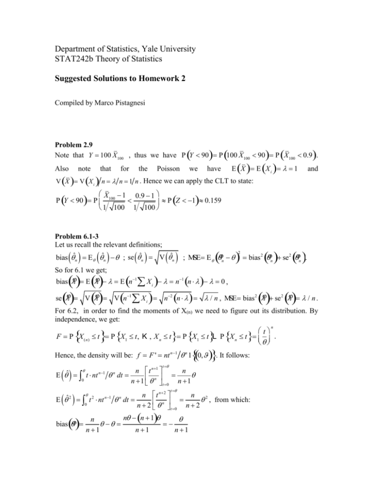
Department of Statistics, Yale University
STAT242b Theory of Statistics
Suggested Solutions to Homework 2
Compiled by Marco Pistagnesi
Problem 2.9
Note that Y  100 X 100 , thus we have P Y  90  P 100 X100  90  P X100  0.9 .

Also
note
 
that
for
  n
V X  V Xi
the
Poisson
 
we
have
 
E X  E X    1

and
i
n  1 n . Hence we can apply the CLT to state:
 X  1 0.9  1 
P Y  90  P  100

  P Z  1  0.159
 1 100 1 100 



Problem 6.1-3
Let us recall the relevant definitions;
bias ˆn  E ˆn   ; se ˆn  V ˆn
 
 
 
 


; MSE E  φn  
  bias φ  se φ .
2
2
2
n
n
So for 6.1 we get;
bias φ  E φ    E n1  X i    n1 n      0 ,


 
se φ V φ V n  X 
1
i
n2
 
n      / n , MSE bias φ se φ  / n .
2
2
For 6.2, in order to find the moments of X(n) we need to figure out its distribution. By
independence, we get:

F  P X ( n)
 
 
 

 . It follows:
Hence, the density will be: f  F '  nt n1  n 1 0,

t 

E ˆ   t  nt
 
E ˆ

n 1
0
2
bias φ 

0
n
t
 t  P X1  t, K , X n  t  P X1  t L P X n  t    .

n  t n 1 
n
 dt 



n 
n  1    t 0 n  1
n
t 
t  nt
2
n 1
n  t n2 
n
 dt 

 2 , from which:

n 
n  2    t 0 n  2
n


n  n  1 
n

  

n 1
n 1
n 1
2
 n 2  n 

n
se φ  E φ  E φ  
  
  
n 1 n  2
 n  2   n 1 

  
2
2
2
2
    
n 
2 2
MSE  

.
 
 n  1  n  1 n  2 
n 1 n  2
For 6.3, similarly we get:
bias φ  E 2 X n    2n1  E X i    2n1 n   2    0 ,

  


 
 



 


se φ  V 2X n  4n2  V X i  4n2 n   2 12  

2

MSE 0  
 
2
3n
2
,
3n
3n .
Problem 7.4
For this problem I will propose a fairly detailed solution, as the vast majority of you
approached it in a slightly imprecise way.
n
Recall that, be definition, Fˆn  x   n1 i 1 I  X i  x  .
We know that X1 , , X n ~ F are iid, and thus we also know that the I  X i  x  are also
iid (note that the indicator is also a random variable). The RHS of the formula above is a
sample average of indicators, and thus the CLT applies to it. In order to apply this
theorem we first must find the mean and variance of each of the identical random
variables I  X i  x  . We simplify those calculations by computing the expectation value
of I to every power:
E I n X i  x  0n  P X i  x  1n  P X i  x  P X i  x  F x . Hence:
 



  E  I  X i  x    F  x  and  2
   
 V I X  x  F x  F x  F x 1 F x 1.

2
i
Now the CLT allows as to make the following one statement and no others:


lim 
n  





 ~ N 0,1




 
F x 1  F x 
φ x  F x
F
n
n
 
(1)
In particular, it does not allow us to state:
1
Note that we could have reached the same conclusion by arguing that the indicator takes
only 2 values with success probability given by F(x), hence is distributed as
Bernoulli(F(x)).
 
 

F x 1 F x 

lim Fφn x ~ N  F x ,
n
n




(2)
I take the chance, once again, for a digression on the very meaning of this fundamental
theorem in Statistics. The random variable to which it applies is (any) sample average,
standardized by its mean and variance. If we do not standardize (in particular by the
variance), we do not get convergence. Hence (2) is wrong as Fφn x is not standardized

there. The key point is that, in order to get convergence, we need to scale the random
quantity by a factor depending on n (for a discussion of what such factor has to be, cfr.
Sugg.sol. for HW1 problem5.1a).
You can look at that from another perspective too: isn’t it suspicious that in (2) n appears
also in the limit? Shouldn’t that limit be, indeed, a limit fixed quantity approached by
Fφn x as n escapes to infinity? Indeed, it should, and (2) is not even a sensible

mathematical expression at all.
So to make the point, some of you argued (2), and that is wrong. Some others, went this
way: from (1) we observe that the finite sample approximate distribution of
Fφn x  F x
is N(0,1), hence
F x 1 F x
 
   
n
 
 

F x 1 F x 
 for n finite!
Fφn x ~ approx N  F x ,
(3)
n


so that (3) is much different from (2) and is not a limiting distribution at all. Almost all of
you that undertook this argument stopped here by saying that (3) is the sought limiting
distribution and this is also wrong. Yet, this second line of thought that brings to (3) is
close to the correct answer, that requires only a further step. (3) gives the approximate
distribution for n finite, so let us just take the limit now for n   . This would be our
limiting distribution, and we see that the variance will shrink to zero and the limiting
distribution degenerates to F(x). We can then conclude that the empirical distribution
function converges in probability to the true one. This result is of great significance and
is, for example, motivation for the Method of Moments2.

2

For the nerds, it can be proved that the convergence is also uniform in the sup norm.
This would be the Glivenko-Cantelli theorem.