Problem 7-1-1
The peak hour traffic volume and the daily traffic volume on a given highway have been observed for 5 days.
Data are as follows:
Day Peak Hour Traffic Daily Traffic
1
2
3
4
1.2
1.0
1.4
0.9
5 0.6
Where all units of traffic volume are in terms of thousand vehicles.
5.0
4.5
6.5
4.6
3.0
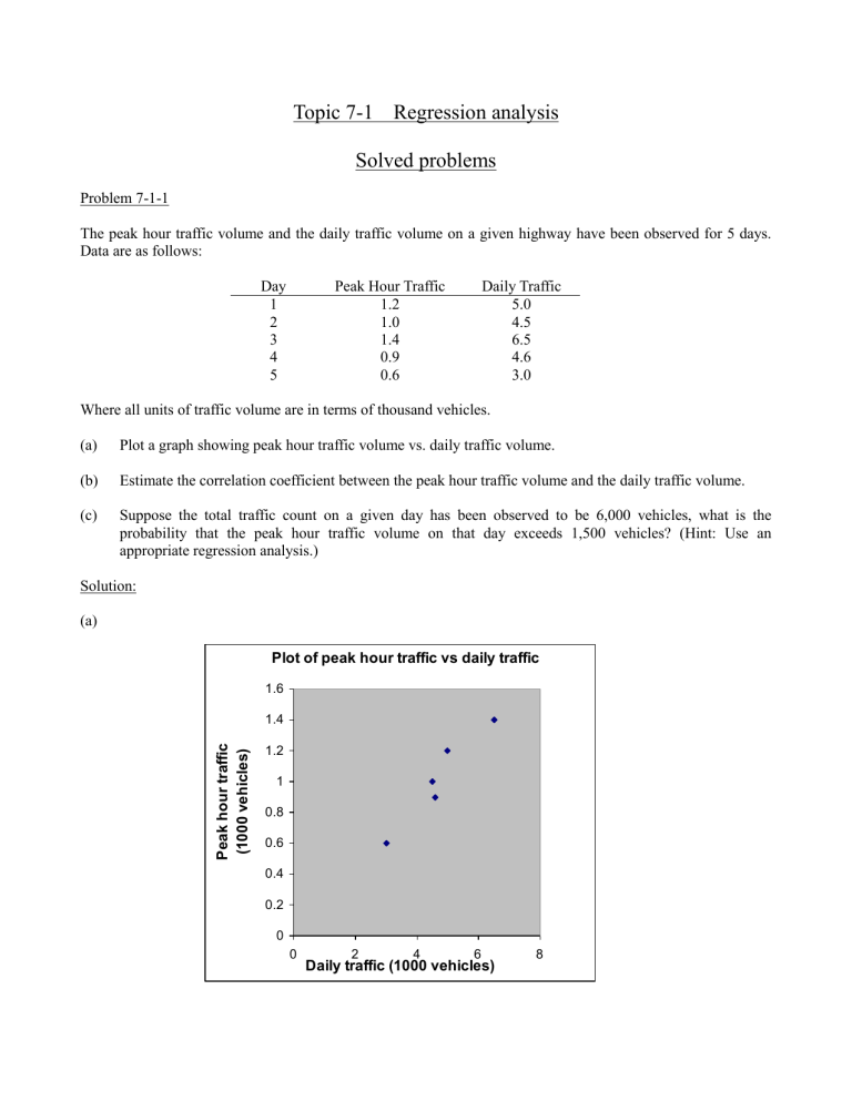
(a) Plot a graph showing peak hour traffic volume vs. daily traffic volume.
(b) Estimate the correlation coefficient between the peak hour traffic volume and the daily traffic volume.
(c) Suppose the total traffic count on a given day has been observed to be 6,000 vehicles, what is the probability that the peak hour traffic volume on that day exceeds 1,500 vehicles? (Hint: Use an appropriate regression analysis.)
Solution:
(a)
Plot of peak hour traffic vs daily traffic
1.6
1.4
1.2
1
0.8
0.6
0.4
0.2
0
0 2 4 6
Daily traffic (1000 vehicles)
8

(b) Let X be the daily traffic volume and Y the peak hour traffic volume, both in thousand vehicles. By Ang
& Tang (7.22), the correlation coefficient between X and Y is estimated by
 n
1

1 n  i

1 x i y i
 n x y s x s y
With n = 5, i n 

1 x i y i
= 25.54, x = 1.02, y = 4.72, and the sample standard deviations s x
= 0.303315018
(c) while s y
= 1.251798706,
 
= (1/4)(1.468 / 0.379689347)

0.967 x i y i
5 1.2 x i y i
6 x i
2 y i
'   ˆ   ˆ x i
(y i
– y i
’) 2
25 1.085577537 0.0130925
4.5
6.5
4.6
3
1
1.4
0.9
0.6
4.5
9.1
4.14
1.8
20.25 0.968474793 0.00099384
42.25 1.436885769 0.00136056
21.16 0.991895341 0.00844475
9 0.61716656 0.00029469
23.6 5.1 25.54 117.66 0.02418634 Sum
Mean 4.72 1.02
Since we know the total (daily) traffic count (X), and want a probability estimate about the peak hour traffic (Y), we need the regression of Y on X, i.e. the best estimates of

and

in the model
E(Y | X = x) =

+
 x
Ang & Tang (7.2) and (7.3) give these as

 i n 

1 x i y i
 n x y
 x i
2 n x
2 i n 

1

= (25.54 - 5

4.72

1.02) / (117.66 – 5

4.72
2 ) = 1.468 / 6.268

0.234, and
 y
  ˆ x = 1.02 – 0.23420549

4.72

– 0.085
Also, by (7.5), using the results in the table above, we estimate the variance of Y (assumed constant)
2
S
Y | x
 n
1

2 i n 

1
( y i
 y i
'
)
2
= 0.02418634 / (5 – 2)

0.008062114
Hence when the daily traffic is 6000 vehicles, i.e. x = 6, Y has the estimated parameters

Y
= –0.085449904 + 0.23420549

6 = 1.319783025


Y
= 0.008062114
0.5
= 0.089789278
Hence the estimated probability of peak hour traffic exceeding 1500 vehicles is
P(Y > 1.5) = 1 – P(Y

1.5)
= 1 – 
(
1 .
5

0.0224

1.31978302
5
0.08978927
8
)
= 1 –

(2.007)
Problem 7-1-2
A survey of a passenger car weight (in kip) and gasoline mileage (in miles per gallon) gives the following:
Car Gasoline Mileage (mpg) Weight (kip)
1
2
3
4
25
17
20
21
2.5
4.2
3.6
3.0
These 4 cars represent a random sample of the entire passenger car population.
(a) Suppose passenger car weight (in kips) is normally distributed, and (by analysis using probability paper) its mean and standard deviation are estimated to be 3.33 and 1.04, respectively. Find the probability that another car picked at random from the population will weigh more than 4.5 kips.
(b) Using linear regression analysis with constant variance, answer the following:
If you buy a car that weighs 2.3 kips, what is the probability that it will have a gasoline mileage of more than 28 mpg?
Solution:
(a) Let X be the car weight in kips; X ~ N(3.33, 1.04). Hence
P(X > 4.5) = P(
X

 

4 .
5

3 .
33
.
04
)
1
= P(Z > 1.125) = 1 –

(1.125) = 1 - 0.869705436

0.130
(b) Let Y be the gasoline mileage. For linear regression, we assume E(Y | X = x) =

+
 x and seek the best (in a least squares sense) estimates of

and

in the model. Based on the following data, x i
(kips) y i
(mpg) x i y i x i
2 y i
'     ˆ x i
(y i
– y i
’) 2
2.5 25 6.25 62.5 24.33641 0.440358 sum average
4.2
3.6
3.0
13.3
3.325
17
20
21
83.0
20.75
17.64
12.96
9.00
45.9
71.4
72
63
268.9
16.94624 0.002891
19.55453 0.198442
22.16283 1.352165
1.993856


 i n 

1 x i y i
 n x y
 x i
2 n x i n 

1
 2
= (45.9 - 4

3.325

20.75) / (268.9 – 4
= 1.468 / 6.268

- 4.35, and

3.325
2 )


 y
  ˆ x = 20.75 – 4.347158218

3.325

35.20
Also, by Ang & Tang (7.5), using the results in the preceding table, we estimate the variance of Y (which is assumed constant)
2
S
Y | x
 n
1

2 i n 

1
( y i
 y i
'
)
2
= 1.993856 / (4 – 2)

0.997
Hence when the car weighs 2.3 kips, i.e. x = 2.3, Y has the estimated parameters

Y
= 35.20430108 + (-4.347158218)

2.3 = 25.20583717

Y
= 0.996927803
0.5
= 0.99846272
Hence the estimated probability of gas mileage being more than 28 mpg is
P(Y > 28) = 1 – P(Y

28)
28

= 1 – 
(
25.2058371
7
)
0.99846272
= 1 –

(2.798) = 1 – 0.997432632

0.00257

Exercise 7-1-1
The error incurred in a given type of measurement by a surveyor appears to be affected by the surveyor’s years of experience. The following is the data observed for 5 surveyors.
Surveyor Years of
Experience, Y
Measurement Error in inches, M
1
2
3
4
5
3
5
10
20
25
1.5
0.8
1.0
0.8
0.5
On the basis of the above information, answer the following and state your assumptions:
(a) For a surveyor with 15 years of experience, what is the probability that his measurement error be less than 1 inch? (Ans. 0.713)
(b) For a 100-year-old surveyor who has 60 years of experience, can you estimate the probability that his measurement error will be less than 1 inch? Please elaborate.
Exercise 7-1-2
The actual concrete strength, Y, in a structure is generally higher than that, X, measured on specimen from the same batch of concrete. Data shows that a regression equation for predicting the actual concrete strength is
E( Y x) = 1.12x + 0.05 (ksi); 0.1 < x < 0.5 and
Var( Y x) = 0.0025 (ksi) 2
Assume that Y follows a normal distribution for a given value of x.
(a) For a given job where the measured strength is 0.35 ksi, what is the probability that the actual strength will exceed the requirement of 0.3 ksi?
(b) Suppose the engineer has lost the data on the measured strength on the concrete specimen. He however recalls that it is either 0.35 or 0.40 with the relative likelihood of 1 to 4. What is the probability that the actual strength will exceed the requirement of 0.3 ksi?
(c) Suppose the measured values of concrete strength at two sites A and B are 0.35 and 0.4 ksi respectively.
What is the probability that the actual strength for the concrete structure at site A will be larger than that at site B? You may assume that the predicted actual concrete strength between sites are statistically independent.
Exercise 7-1-3

Data on the construction costs of 3 houses in a given residential area are as follows:
Floor Area (1000 sq. ft.)
1.05
1.83
Cost ($1,000)
63
92
3.14
Plot the above data on a piece of graph paper.
204
(a) Determine by linear regression the relation between construction cost of houses as a function of floor area. Sketch this on the graph.
(b) Estimate the standard deviation of construction cost for given floor area.
(c) How good is the linear relation between cost and floor area (i.e., answer this by evaluating the correlation coefficient)?
(d) If you wish to build a house with 2500 sq. ft. of floor area, what is the probability that the construction cost will not exceed $180,000 (based on the information given above)? Assume that the cost for a given floor area is normally distributed.