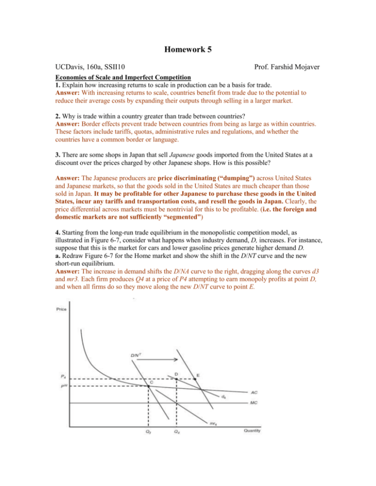
Homework 5
UCDavis, 160a, SSII10
Prof. Farshid Mojaver
Economies of Scale and Imperfect Competition
1. Explain how increasing returns to scale in production can be a basis for trade.
Answer: With increasing returns to scale, countries benefit from trade due to the potential to
reduce their average costs by expanding their outputs through selling in a larger market.
2. Why is trade within a country greater than trade between countries?
Answer: Border effects prevent trade between countries from being as large as within countries.
These factors include tariffs, quotas, administrative rules and regulations, and whether the
countries have a common border or language.
3. There are some shops in Japan that sell Japanese goods imported from the United States at a
discount over the prices charged by other Japanese shops. How is this possible?
Answer: The Japanese producers are price discriminating (“dumping”) across United States
and Japanese markets, so that the goods sold in the United States are much cheaper than those
sold in Japan. It may be profitable for other Japanese to purchase these goods in the United
States, incur any tariffs and transportation costs, and resell the goods in Japan. Clearly, the
price differential across markets must be nontrivial for this to be profitable. (i.e. the foreign and
domestic markets are not sufficiently “segmented”)
4. Starting from the long-run trade equilibrium in the monopolistic competition model, as
illustrated in Figure 6-7, consider what happens when industry demand, D, increases. For instance,
suppose that this is the market for cars and lower gasoline prices generate higher demand D.
a. Redraw Figure 6-7 for the Home market and show the shift in the D/NT curve and the new
short-run equilibrium.
Answer: The increase in demand shifts the D/NA curve to the right, dragging along the curves d3
and mr3. Each firm produces Q4 at a price of P4 attempting to earn monopoly profits at point D,
and when all firms do so they move along the new D/NT curve to point E.
b. From the new short-run equilibrium, is there exit or entry of firms, and why?
Answer: In the short-run with trade, monopoly profits are positive because price exceeds average
cost. As a result, firms enter the industry and NT increases.
c. Describe where the new long-run equilibrium occurs, and explain what has happened to the
number of firms and the prices they charge.
Answer: In the long-run with trade, firm entry shifts D/NT and d4 to the left and makes d4 more
elastic until it is tangent to the average cost curve. At that point, monopoly profits are zero and
firms no longer enter the industry. Relative to the short-run equilibrium in (b), the number of
firms increases and price decreases.
5. Our derivation of the gravity equation from the monopolistic competition model used the
following logic:
(1) Each country produces many products;
(2) Each country demands all of the products that every other country produces;
(3) Thus, large countries demand more imports from other countries.
The gravity equation relationship does not hold in the Heckscher-Ohlin model. Explain how the
logic of the gravity equation breaks down in the Heckscher-Ohlin model: that is, which of the
above statements is no longer true in the Heckscher-Ohlin model?
Answer: The Heckscher-Ohlin model assumes perfect competition. Therefore, each country
produces many products. However, in the Heckscher-Ohlin model not all products produced in
other countries (in autarky) are imported under trade. Rather, because products are not
differentiated, only those identical products with a lower relative price abroad are imported, and
countries specialize in the good that uses their abundant factor intensively. Hence larger countries
do not necessarily demand more imports from other countries.
6. The United States, France, and Italy are among the world’s largest producers. To answer the
following questions, assume that their markets are monopolistically competitive, and use the
gravity equation with B = 93 and n = 1.25.
a. Using the gravity equation, compare the expected level of trade between the United States and
France and between the United States and Italy.
Answer: The expected level of trade between the United States and France is
10(1,830 * 12,409) / 5,544125 = $4,747 billion. The expected level of trade between the United
States and Italy is 10(1,668 * 12,409) / 6,229125 = $3,740 billion.
(Note: These numbers are larger than is realistic because we are using the gravity equation
estimated on the United States and Canada state/provincial trade, rather than the equation
estimated on international trade.)
b. The distance between Paris and Rome is 694 miles. Would you expect more French trade with
Italy or with the United States? Explain what variable (i.e., country size or distance) drives your
result.
Answer: The expected level of trade between Italy and France is 10(1,830 * 1,668) / 694125 =
$8,569 billion. This number is so large because it reflects the short distance between the two
countries. In particular, this number is larger than the predicted amount of trade between the
United States and Italy, as calculated in part (a).
7. What evidence is there that Canada is better off under the free-trade agreement with the United
States?
Answer: Economist Daniel Trefler found that between 1988 and 1996 the productivity of
Canadian firms increased by as much as 15% in industries most affect by the tariff cuts. The
growth in productivity translates to an increase in real earnings of 3% over the 8-year period.
Moreover, Canadian consumers gained from the fall in prices and the rise in product variety.
8. Consider the long-run trade equilibrium in the monopolistic competition model as illustrated
below. Consider a situation where the foreign and domestic demand for a particular good
increase. For instance, suppose that this is the market for cars and lower gasoline prices generates
higher demand.
a) Redraw the Figure below and show what happens when this change in demand occurs.
Specifically, show which curve(s) shift.
b) If the old equilibrium is at point C, describe where the new long run equilibrium occurs, and
what has happened to the number of firms and the price they charge.
D0/Nc
C’
C
dc
mrc
dc’
AC
MC
mrc’
Short run effect: Demand goes up and so does price and the scale of production. The existing
firms make above normal profits as the number of firms are fixed in the short run.
Nd >Nc
D0/Nc
D1/Nd
C
D
dc
mrd
dc’
AC
MC
Long Run effect: Higher profit attracts new firms to the market. As new firms enter the market
demand curve facing each firm shifts down. Consequently the price and the scale of production
fall. But now there are more varieties in the market and demand curve is flatter.
9. Suppose the Home firm is considering whether to enter the Foreign market. Assume that the
Home firm has the following costs and demand:
Fixed Costs = $140
Marginal Costs = $10/unit
Local Price = $25
Local Quantity = 20
Export Price = $15
Export Quantity = 10
a. Calculate the firm’s total costs from selling only in the local market.
Answer:
Total Costs = $10 . 20 + $140 = $340
Variable Fixed
Costs
Costs
b. What is the firm’s average cost from selling only in the local market?
Answer:
$340/20 = $17
Total
Average
Costs
Costs
c. Calculate the firm’s profit from selling only in the local market.
Answer:
$25 . 20 – $340 = $160
Revenue Total Profit
Costs
d. Should the Home firm enter the Foreign market? Briefly explain why.
Answer: The firm should enter the Foreign market because it would be earning an additional $50.
The firm is able to earn the extra profit because the exporting price, $15, although lower than the
average costs, $17, is higher than the marginal cost of $10.
e. Calculate the firm’s profit from selling to both markets.
Answer:
($25 . 20 + $15 . 10) - $10 . 30 - $140 = $210
Revenue
Fixed Variable Profits
Costs
Costs
f. Is the Home firm dumping? Briefly explain.
Answer: The firm is dumping because its export price ($15) is lower than its local price ($25).
10. Suppose consumers at Home have the following demand:
P = 50 – 0.5Q
a. Write the Home monopolist’s marginal revenue equation.
Answer:
TR=P.Q = 50 Q – 0.5Q2
MR =50 – Q
b. Assuming that marginal costs and average costs both equal $10 per unit, what is the firm’s
profit-maximizing level of output and price?
Answer:
MR = MC
50 - Q = 10
Q = 40
P = 50 - .5(40) = 30
c. Calculate the Home firm’s profit.
Answer:
$30 . 40 - $10 . 40 = $800
Revenue Variable Profits
Costs