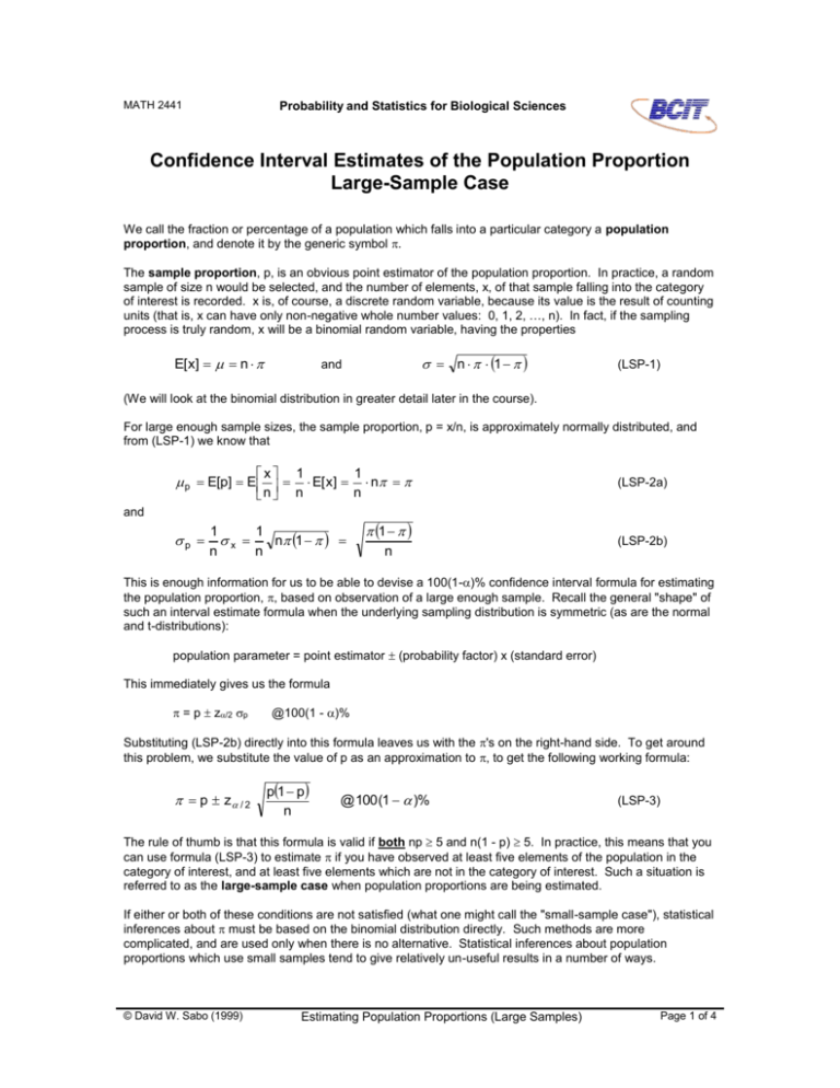
MATH 2441
Probability and Statistics for Biological Sciences
Confidence Interval Estimates of the Population Proportion
Large-Sample Case
We call the fraction or percentage of a population which falls into a particular category a population
proportion, and denote it by the generic symbol .
The sample proportion, p, is an obvious point estimator of the population proportion. In practice, a random
sample of size n would be selected, and the number of elements, x, of that sample falling into the category
of interest is recorded. x is, of course, a discrete random variable, because its value is the result of counting
units (that is, x can have only non-negative whole number values: 0, 1, 2, …, n). In fact, if the sampling
process is truly random, x will be a binomial random variable, having the properties
E[ x]    n  
  n    1   
and
(LSP-1)
(We will look at the binomial distribution in greater detail later in the course).
For large enough sample sizes, the sample proportion, p = x/n, is approximately normally distributed, and
from (LSP-1) we know that
x
1
1
 p  E[p]  E     E[ x]   n  
n
n  n
and
p 
1
1
x 
n 1    
n
n
 1   
n
(LSP-2a)
(LSP-2b)
This is enough information for us to be able to devise a 100(1-)% confidence interval formula for estimating
the population proportion, , based on observation of a large enough sample. Recall the general "shape" of
such an interval estimate formula when the underlying sampling distribution is symmetric (as are the normal
and t-distributions):
population parameter = point estimator  (probability factor) x (standard error)
This immediately gives us the formula
 = p  z/2 p
@100(1 - )%
Substituting (LSP-2b) directly into this formula leaves us with the 's on the right-hand side. To get around
this problem, we substitute the value of p as an approximation to , to get the following working formula:
  p  z / 2
p1  p
n
@ 100 (1   )%
(LSP-3)
The rule of thumb is that this formula is valid if both np  5 and n(1 - p)  5. In practice, this means that you
can use formula (LSP-3) to estimate  if you have observed at least five elements of the population in the
category of interest, and at least five elements which are not in the category of interest. Such a situation is
referred to as the large-sample case when population proportions are being estimated.
If either or both of these conditions are not satisfied (what one might call the "small-sample case"), statistical
inferences about  must be based on the binomial distribution directly. Such methods are more
complicated, and are used only when there is no alternative. Statistical inferences about population
proportions which use small samples tend to give relatively un-useful results in a number of ways.
© David W. Sabo (1999)
Estimating Population Proportions (Large Samples)
Page 1 of 4
Reasonable precision and reliability in estimating population proportions almost certainly requires the use of
large samples.
Example 1: In a letter to the editor (Nature, 396, p. 531) discussing an earlier report of increased
susceptibility to cervical cancer by women who were homozygous at codon-72 of the p53 gene, A. M.
Josefson and her coauthors reported on frequencies of the Pro/Pro, Pro/Arg and Arg/Arg codons. They
found that 246 out of a sample of 626 women with no diagnosis of cervical cancer were heterozygous at this
site. Compute a 95% confidence interval estimate of the proportion of all cancer-free women who are
heterozygous at this site, based on this sample data.
Solution:
The proportion of women in the sample who were heterozygous at this site is simply
p
246
 0.393
626
Since in the sample of 626 women, there were 246 who were heterozygous, there must have been
626 - 246 = 380 women who were not heterozygous (ie. homozygous). Since both of these numbers are
bigger than 5, we are justified in using the large-sample formulas given above. For a 95% confidence
interval estimate, we need z.025 = 1.96. Thus, the required estimate is
  0.393  1.96
(0.393 )(1  0.393 )
626
 0.393  0.038
@ 95%
You could also write this is the form
0.355    0.431 @95%
indicating that there is a probability of 0.95 that the interval 35.5% to 43.1% has captured the value of the
actual proportion of the population of all women without cancer who are heterozygous at this site.

Deciding on Appropriate Sample Sizes
As with confidence interval estimates in general, the confidence interval estimates of the population
proportion given by formula (LSP-3) above contains an "uncertainty" term which represents the precision of
the estimate, and which has a value dependent on both the value of the population proportion, and the
sample size. The appropriate sample size to use is thus determined in part by the precision desired in the
estimate to be obtained and in part by what one expects the value of the population proportion may be.
To obtain an interval estimate with a precision of, say, , we need to select a sample of size n, where n
satisfies the following equation:
z / 2
 1   
n
 z / 2
p1  p

n
(The exact equation is the one with 's on the left-hand side, but in the confidence interval formula given
earlier, we approximate  by the known value of p. However, before the sampling has been done, we don't
have a value for either  or p, so it doesn't much matter which of these two equations you work with.)
Solving for n, we get
n
Page 2 of 4
z 2 / 2  1   
2
Estimating Population Proportions (Large Samples)
(LSP-4)
© David W. Sabo (1999)
All that remains is to decide what to do about the unknown  on the right-hand side here. There are two
distinct approaches.
First, you could carry out a relatively small pilot study, and use the sample proportion, p, that you get from
that data as a rough estimate of  in formula (LSP-4).
Example 1a: Approximately what size of sample would the researchers described in Example 1 above had
to have used if they wished to get a 95% confidence interval estimate of the proportion of heterozygous
women which was accurate to within 0.01 (or 1 percentage point). You may use the fact that the population
proportion appears to be approximately equal to 0.40 based on the reported studies.
Solution:
We are asked to recommend a minimum value of n given  = 0.01 and   0.40. Substituting these values
and the value z.025 = 1.96 into formula (LSP-4), we get
n
1.96 2  0.40  0.60
0.012
 9219 .84
This indicates they would have to sample 9220 or more women to be able to achieve the stated precision of
estimate. What's worse, even if they include 9220 women in their sample, they could still miss their target
precision if the resulting value of p was not 0.40. For example, if after sampling 9220 women, they obtained
a sample proportion equal to, say, 0.43 (which is near the upper end of the confidence interval estimate
obtained in Example 1, and so is not beyond the realm of possibility), then their new estimate of  would turn
out to be:
  0.430  1.96
(0.430 )(1  0.430 )
9220
 0.430  0.0101
@ 95%
The '' term here is not a great deal larger than 0.01 (in fact, this overage would probably be of no practical
significance at all in real work), but still, it is larger than 0.01. The estimate of 9220 as a required sample
size was not a guarantee.

There is a second approach to estimating appropriate
sample size: we could call it the pessimistic
approach. The difficulty here is that the value of n
given by (LSP-4) is directly proportional to (1 - ).
The bigger the value of this product, the bigger the
required value of n to achieve a target value for .
However, by looking at a graph of y = (1 - ) as a
function of , you can see that this product has a
maximum value that occurs when  = 0.5. The
uncertainty term in the confidence interval formula is
largest when  =0.5, and so if we pick n to achieve a
certain value of  when  =0.5, we will be guaranteed
that the uncertainty term will be less than or equal to
that value of  regardless of the value of p obtained
from the sample. Thus, the pessimistic approach
says: use n given by the first whole number larger than
0.25  z 2 / 2
2
y = (1-)
0.25
0.20
0.10

0
0.5
1
(LSP-5)
Example 1b: What sample size is suggested for the study described in Example 1 if we use this most
pessimistic approach, but still wish to get a 95% confidence interval estimate precise to the nearest 0.01?
© David W. Sabo (1999)
Estimating Population Proportions (Large Samples)
Page 3 of 4
Solution:
Just plug z.025 = 1.96 and  = 0.01 into (LSP-5) and round up to the nearest whole number:
0.25  1.96 2
0.012
 9604
Actually, no rounding was necessary here. Thus, if a sample of size 9604 was used, the estimate of  is
guaranteed to come out precise to within 0.01 or 1 percentage point.
The disadvantage of the pessimistic approach is that, of course, you may end up collecting data from a far
larger sample than was necessary, which would normally mean that you spent more money on the study
than was necessary. For instance, if the sample of size 9604 was found to have a proportion of 0.400
women who were heterozygous at this site on the p53 gene, then the interval estimate of  would turn out to
be
  0.400  1.96 
0.400  0.600
 0.400  0.0098
9604
@ 95 %
It's not so much that this is slightly more precise than was desired, but that this small (and unnecessary)
additional precision required sampling nearly 400 extra individuals.

One last comment before leaving this issue of sample sizes: notice that for populations that are fairly evenly
split between two categories,   0.5, we require really quite large samples in order to achieve 1 percentage
point accuracy at a 95% confidence level. From looking at the graph just above, you may think this will not
be as big a problem for values of  near zero or 1. For values near 1, it isn't, but for values near zero, the
problem is even worse to get the same relative precision. For this reason, it is relatively rare to attempt
estimates of population proportions which are much more precise than 0.03 or 0.04, unless some unusual
aspects of the experiment require higher precision. (You may notice that when newscasters report the
results of political polls, they often explain that the numbers they give are "accurate to within 4 percentage
points, 19 times out of 20"  this means the sampling provided a 95% confidence interval estimate with a
precision of 0.04.)
Page 4 of 4
Estimating Population Proportions (Large Samples)
© David W. Sabo (1999)