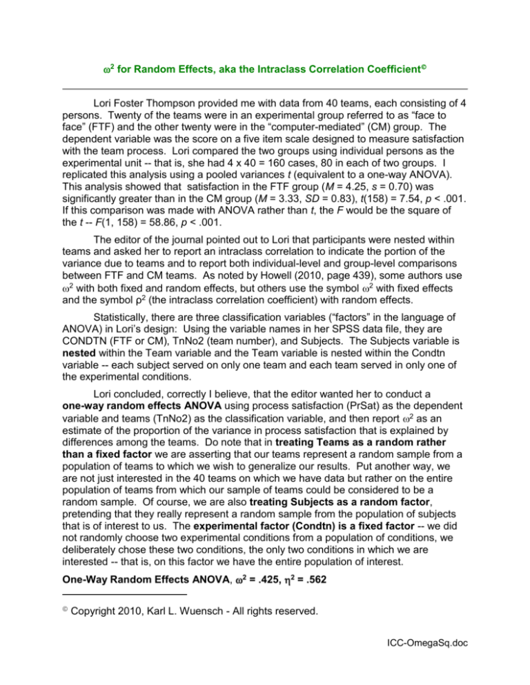
2 for Random Effects, aka the Intraclass Correlation Coefficient
Lori Foster Thompson provided me with data from 40 teams, each consisting of 4
persons. Twenty of the teams were in an experimental group referred to as “face to
face” (FTF) and the other twenty were in the “computer-mediated” (CM) group. The
dependent variable was the score on a five item scale designed to measure satisfaction
with the team process. Lori compared the two groups using individual persons as the
experimental unit -- that is, she had 4 x 40 = 160 cases, 80 in each of two groups. I
replicated this analysis using a pooled variances t (equivalent to a one-way ANOVA).
This analysis showed that satisfaction in the FTF group (M = 4.25, s = 0.70) was
significantly greater than in the CM group (M = 3.33, SD = 0.83), t(158) = 7.54, p < .001.
If this comparison was made with ANOVA rather than t, the F would be the square of
the t -- F(1, 158) = 58.86, p < .001.
The editor of the journal pointed out to Lori that participants were nested within
teams and asked her to report an intraclass correlation to indicate the portion of the
variance due to teams and to report both individual-level and group-level comparisons
between FTF and CM teams. As noted by Howell (2010, page 439), some authors use
2 with both fixed and random effects, but others use the symbol 2 with fixed effects
and the symbol ρ2 (the intraclass correlation coefficient) with random effects.
Statistically, there are three classification variables (“factors” in the language of
ANOVA) in Lori’s design: Using the variable names in her SPSS data file, they are
CONDTN (FTF or CM), TnNo2 (team number), and Subjects. The Subjects variable is
nested within the Team variable and the Team variable is nested within the Condtn
variable -- each subject served on only one team and each team served in only one of
the experimental conditions.
Lori concluded, correctly I believe, that the editor wanted her to conduct a
one-way random effects ANOVA using process satisfaction (PrSat) as the dependent
variable and teams (TnNo2) as the classification variable, and then report 2 as an
estimate of the proportion of the variance in process satisfaction that is explained by
differences among the teams. Do note that in treating Teams as a random rather
than a fixed factor we are asserting that our teams represent a random sample from a
population of teams to which we wish to generalize our results. Put another way, we
are not just interested in the 40 teams on which we have data but rather on the entire
population of teams from which our sample of teams could be considered to be a
random sample. Of course, we are also treating Subjects as a random factor,
pretending that they really represent a random sample from the population of subjects
that is of interest to us. The experimental factor (Condtn) is a fixed factor -- we did
not randomly choose two experimental conditions from a population of conditions, we
deliberately chose these two conditions, the only two conditions in which we are
interested -- that is, on this factor we have the entire population of interest.
One-Way Random Effects ANOVA, 2 = .425, 2 = .562

Copyright 2010, Karl L. Wuensch - All rights reserved.
ICC-OmegaSq.doc
Page 2
David Howell (2007, page 328) points out that “one version of the intraclass
correlation coefficient is nothing but 2 for the random model.” On pages 414 through
415, he shows how to compute 2 for one-way through three-way designs, including the
one-way random design, which I describe here:
(MSA  MSE ) / n
, where MSA is the mean square among teams, MSE is the
MSE  (MSA  MSE ) / n
error (within teams) mean square, and n is the number of scores in each team. In the
seventh edition of Howell’s Methods text only two-way ANOVA is included, but he
provides a link to a table of expected mean squares for three-way designs.
2 
Now I obtain the random effects ANOVA, using my preferred statistical program,
SAS. Here is the procedural code I used, followed by the output:
proc glm; class tm_no2; model prsat = tm_no2; random tm_no2 / test; run;
-----------------------------------------------------------------------------------------------The SAS System
2
The GLM Procedure
Dependent Variable: PRSAT
Source
DF
Sum of
Squares
Mean Square
F Value
Pr > F
Model
39
71.1840000
1.8252308
3.96
<.0001
Error
120
55.3600000
0.4613333
Corrected Total
159
126.5440000
R-Square
Coeff Var
Root MSE
PRSAT Mean
0.562524
17.92125
0.679215
3.790000
Source
DF
Type III SS
Mean Square
F Value
Pr > F
TM_NO2
39
71.18400000
1.82523077
3.96
<.0001
-----------------------------------------------------------------------------------------------The SAS System
4
The GLM Procedure
Tests of Hypotheses for Random Model Analysis of Variance
Dependent Variable: PRSAT
Source
DF
Type III SS
Mean Square
F Value
Pr > F
TM_NO2
39
71.184000
1.825231
3.96
<.0001
Error: MS(Error)
120
55.360000
0.461333
------------------------------------------------------------------------------------------------
For a one-way ANOVA, the basic analysis for the random effect model is
identical to that for the fixed effect model. The computation of the 2 does differ,
Page 3
however, between the fixed effect model and the random effect model. Computation of
the 2 for this analysis is:
2 
(MSA  MSE ) / n
(1.825  0.461) / 4
0.341


 0.425 .
MSE  (MSA  MSE ) / n 0.461  (1.825  0.461) / 4 0.802
Omega-squared is considered to be superior to eta-squared for estimating the
proportion of variance accounted for by an ANOVA factor. Eta-squared tends to
overestimate that proportion -- but eta-squared is certainly easier to compute:
2 
SSEffect
71.184

 0.563 . Notice that this is the R2 reported by SAS.
SSTotal
126.544
One-Way Fixed Effects ANOVA, 2 = .419, 2 = .563
For pedagogical purposes, I’ll show the computation of 2 treating teams as a
fixed variable. The estimated treatment variance is
(a  1)(MSA  MSE ) (40  1)(1.825  0.461)

 0.332. The term “a” is the number of
(n)(a)
(4)( 40)
levels of the team variable. The estimated total variance is equal to the estimated
treatment variance plus the estimated error variance, .332  MSE  .332  .461  .793.
.332
 .419 .
Accordingly,  2 
.793
Two-Way Mixed Effects ANOVA
One should keep in mind that the 2 for teams, as computed above, includes the
effect of the experimental treatment, Condtn -- that is, we have estimated the variance
among the teams, but part of that variance is due to the fact that the two experimental
groups of teams were treated differently, and the other part of it is due to other
differences among teams (error, effects of extraneous variables, reflected in differences
among subjects’ scores within teams).
If one wanted to determine the variance of teams after excluding variance due to
the experimental condition, a mixed factorial ANOVA, Condtn x Teams (nested within
Condtn), could be conducted. Here is the SAS code and output for such an analysis,
treating Condtn as fixed and Teams as random:
proc glm; class condtn tm_no2; model prsat = condtn tm_no2(condtn);
random tm_no2(condtn) / test; run;
-----------------------------------------------------------------------------------------------The SAS System
6
The GLM Procedure
Dependent Variable: PRSAT
Source
DF
Sum of
Squares
Mean Square
F Value
Pr > F
Model
39
71.1840000
1.8252308
3.96
<.0001
Error
120
55.3600000
0.4613333
Page 4
Corrected Total
159
126.5440000
R-Square
Coeff Var
Root MSE
PRSAT Mean
0.562524
17.92125
0.679215
3.790000
Source
DF
Type III SS
Mean Square
F Value
Pr > F
CONDTN
TM_NO2(CONDTN)
1
38
33.48900000
37.69500000
33.48900000
0.99197368
72.59
2.15
<.0001
0.0009
-----------------------------------------------------------------------------------------------The SAS System
8
The GLM Procedure
Tests of Hypotheses for Mixed Model Analysis of Variance
Dependent Variable: PRSAT
PRSAT
Source
DF
Type III SS
Mean Square
F Value
Pr > F
CONDTN
1
33.489000
33.489000
33.76
<.0001
Error
Error: MS(TM_NO2(CONDTN))
38
37.695000
0.991974
Source
DF
Type III SS
Mean Square
F Value
Pr > F
TM_NO2(CONDTN)
38
37.695000
0.991974
2.15
0.0009
120
55.360000
0.461333
Error: MS(Error)
Note that the SS for Teams from the previous analysis, 71.184, has been
partitioned into a SS for Condtn, 33.489, and a SS for Teams within conditions, 37.695.
The Total SS (126.544) is comprised of the SS for Condtn, 33.489, plus the SS for
Teams within conditions, 37.695, plus the SS for Subjects within teams within
conditions, 55.36. Do note that the analysis above uses the variance for teams within
conditions as the error variance for testing the effect of Condtn.
The 2 for the entire effect of teams is 71.184/126.544 = .563. That part due to
the experimental manipulation is 33.489/126.544 = .265.
References
Howell, D. C. (2007). Statistical methods for psychology (6th ed.). Belmont, CA:
Thompson Wadsworth.
Howell, D. C. (2010). Statistical methods for psychology (7th ed.). Belmont, CA:
Cengage Wadsworth.
Return to Wuensch’s Statistics Lessons Page
Copyright 2010, Karl L. Wuensch - All rights reserved.