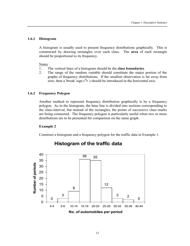
Chapter 1: Descriptive Statistics
1.6.1
Histogram
A histogram is usually used to present frequency distributions graphically. This is
constructed by drawing rectangles over each class. The area of each rectangle
should be proportional to its frequency.
Notes :
1.
The vertical lines of a histogram should be the class boundaries.
2.
The range of the random variable should constitute the major portion of the
graphs of frequency distributions. If the smallest observation is far away from
zero, then a 'break' sign ( ) should be introduced in the horizontal axis.
1.6.2
Frequency Polygon
Another method to represent frequency distribution graphically is by a frequency
polygon. As in the histogram, the base line is divided into sections corresponding to
the class-interval, but instead of the rectangles, the points of successive class marks
are being connected. The frequency polygon is particularly useful when two or more
distributions are to be presented for comparison on the same graph.
Example 2
Construct a histogram and a frequency polygon for the traffic data in Example 1.
Histogram of the traffic data
40
36
35
Number of periods
35
30
25
20
15
12
9
10
5
3
3
0
2
0
0
0-4
5-9
10-14 15-19
20-24
25-29 30-34
No. of automobiles per period
13
35-39 40-44
Chapter 1: Descriptive Statistics
Frequency polygon for the traffic data
Number of periods
40
35
30
25
20
15
10
5
0
0
10
20
30
40
No. of automobiles per period
1.6.3
Frequency Curve
A frequency curve can be obtained by smoothing the frequency polygon.
1.6.4
Cumulative Frequency Distribution and Cumulative Polygon
Sometimes it is preferable to present data in a cumulative frequency distribution,
which shows directly how many of the items are less than, or greater then, various
values.
Less than
4.5
9.5
14.5
19.5
24.5
29.5
34.5
39.5
Cumulative frequency
0
3
12
48
83
95
98
100
14
Chapter 1: Descriptive Statistics
Example 3
Construct a “Less-than” ogive of the distribution of traffic data.
"Less-than" ogive
Cumulative number of
periods
120
100
80
60
40
20
0
0
5
10
15
20
25
30
35
40
No. of automobiles per period (Less than)
1.6.5
Cumulative Frequency Curve
A cumulative frequency curve can similarly be drawn.
1.6.6
Relative Frequency
Relative frequency of a class is defined as:
Frequency of the Class
Total Frequency
If the frequencies are changed to relative frequencies, then a relative frequency
histogram, a relative frequency polygon and a relative frequency curve can similarly
be constructed.
Relative frequency curve can be considered as probability curve if the total area
under the curve be set to 1. Hence the area under the relative frequency curve
between a and b is the probability between interval a and b.
15
Chapter 1: Descriptive Statistics
Example 4
Construct a relative frequency distribution and a percentage distribution from the
traffic data in Example 1.
1.7
Central Tendency
When we work with numerical data, it seems apparent that in most set of data there is a
tendency for the observed values to group themselves about some interior values; some
central values seem to be the characteristics of the data. This phenomenon is referred to as
central tendency. For a given set of data, the measure of location we use depends on what
we mean by middle; different definitions give rise to different measures. We shall consider
some more commonly used measures, namely arithmetic mean, median and mode. The
formulas in finding these values depends on whether they are ungrouped data or grouped
data.
1.7.1
Arithmetic Mean
The arithmetic mean, , or simply called mean, is obtained by adding together all of
the measurements and dividing by the total number of measurements taken.
Mathematically it is given as

 f x
f
i
i
i
16
Chapter 1: Descriptive Statistics
Where -
for grouped data:
fi - is the frequency in the ith class,
xi - is the class mark in the ith class;
for ungrouped data: fi - is the frequency in the ith datum,
xi - is the value in the ith datum.
Arithmetic mean can be used to calculate any numerical data and it is always unique.
It is obvious that extreme values affect the mean. Also, arithmetic mean ignores the
degree of importance in different categories of data.
Example 5
Given the following set of ungrouped data:
20, 18, 15, 15, 14, 12, 11, 9, 7, 6, 4, 1
Find the mean of the ungrouped data.
mean 

20  18  2  15  14  12  11  9  7  6  4  1
12
132
12
 11
1.7.2
Weighted Arithmetic Mean
In order to consider the importance of some data, different weighting factors, wi , can
be assigned to individual datum. Hence the weighted arithmetic mean, , is given as:
17
Chapter 1: Descriptive Statistics

 f w x
 f w
i
i
i
Where
1.7.3
i
i
wi is the weight for the ith datum.
fi and xi are defined same as those in the arithmetic mean for
ungrouped and grouped data.
Median
Median is defined as the middle item of all given observations arranged in order. For
ungrouped data, the median is obvious. In case of the number of measurements is
even, the median is obtained by taking the average of the middle.
Example 6
The median of the ungrouped data:: 20, 18, 15, 15, 14, 12, 11, 9, 7, 6, 4, 1 is
12  11
2
= 11.5
For grouped data, the median can be found by first identify the class containing the
median, then apply the following formula:
n
C
2
median  l1 
(l2  l1 )
fm
where:
l1
n
C
fm
l2
is the lower class boundary of the median class;
is the total frequency;
is the cumulative frequency just before the median class;
is the frequency of the median;
is the upper class boundary containing the median.
It is obvious that the median is affected by the total number of data but is independent
of extreme values. However if the data is ungrouped and numerous, finding the
median is tedious. Note that median may be applied in qualitative data if they can be
ranked.
18