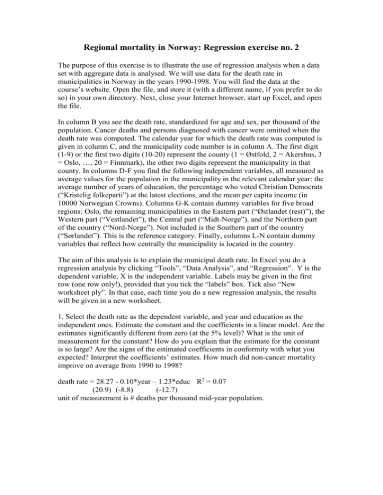
Regional mortality in Norway: Regression exercise no. 2
The purpose of this exercise is to illustrate the use of regression analysis when a data
set with aggregate data is analysed. We will use data for the death rate in
municipalities in Norway in the years 1990-1998. You will find the data at the
course’s website. Open the file, and store it (with a different name, if you prefer to do
so) in your own directory. Next, close your Internet browser, start up Excel, and open
the file.
In column B you see the death rate, standardized for age and sex, per thousand of the
population. Cancer deaths and persons diagnosed with cancer were omitted when the
death rate was computed. The calendar year for which the death rate was computed is
given in column C, and the municipality code number is in column A. The first digit
(1-9) or the first two digits (10-20) represent the county (1 = Østfold, 2 = Akershus, 3
= Oslo, …, 20 = Finnmark), the other two digits represent the municipality in that
county. In columns D-F you find the following independent variables, all measured as
average values for the population in the municipality in the relevant calendar year: the
average number of years of education, the percentage who voted Christian Democrats
(“Kristelig folkeparti”) at the latest elections, and the mean per capita income (in
10000 Norwegian Crowns). Columns G-K contain dummy variables for five broad
regions: Oslo, the remaining municipalities in the Eastern part (“Østlandet (rest)”), the
Western part (“Vestlandet”), the Central part (“Midt-Norge”), and the Northern part
of the country (“Nord-Norge”). Not included is the Southern part of the country
(“Sørlandet”). This is the reference category. Finally, columns L-N contain dummy
variables that reflect how centrally the municipality is located in the country.
The aim of this analysis is to explain the municipal death rate. In Excel you do a
regression analysis by clicking “Tools”, “Data Analysis”, and “Regression”. Y is the
dependent variable, X is the independent variable. Labels may be given in the first
row (one row only!), provided that you tick the “labels” box. Tick also “New
worksheet ply”. In that case, each time you do a new regression analysis, the results
will be given in a new worksheet.
1. Select the death rate as the dependent variable, and year and education as the
independent ones. Estimate the constant and the coefficients in a linear model. Are the
estimates significantly different from zero (at the 5% level)? What is the unit of
measurement for the constant? How do you explain that the estimate for the constant
is so large? Are the signs of the estimated coefficients in conformity with what you
expected? Interpret the coefficients’ estimates. How much did non-cancer mortality
improve on average from 1990 to 1998?
death rate = 28.27 - 0.10*year – 1.23*educ R2 = 0.07
(20.9) (-8.8)
(-12.7)
unit of measurement is # deaths per thousand mid-year population.
2. Add percentage Christian Democrats (column E), mean income (F), and whether or
not the municipality is Oslo (G) as extra independent variables. The high estimate for
Oslo must be caused by other factors than the age composition of Oslo’s population
(controlled for by standardization), the educational level of the population, the
percentage voting Christian Democrats, and the mean income (all three included as
independent variables). Can you think of any explanation?
Coefficients
Intercept
22.57
year
-0.04
educ
-1.16
% Chr. Dem.
-0.05
Income
-0.09
Oslo
1.69
t Stat
12.0
-2.3
-10.7
-12.1
-2.9
2.8
R2 = 0.11
3. Add all other regional dummy variables to the set of independent variables. Before
you include the Central/Periphery/Cen/Per variables, you should choose one of these
three variables as the reference category. The simplest way to do that is to select the
variable in the last column (Cen/Per in column N) as the reference category.
Describe the regional mortality pattern that emerges. Why is the positive effect of
Oslo much lower, and no longer significant, compared to the previous regression
results (Hint: check the reference category)? Do the Central/Periphery variables
contribute significantly to the explanation of the death rate? And how would these
contributions change if you exclude the regional dummy variables in columns G
(Oslo) to K (Northern Norway) from the set of independent variables?
Intercept
year
educ
% Chr. Dem.
Income
Oslo
Østlandet (rest)
Vestlandet
Midt-Norge
Nord-Norge
Central
Periphery
R2 = 0.16
Coefficients
22.76
-0.08
-0.80
-0.04
-0.02
0.51
-0.73
-1.21
-1.05
-0.10
-0.09
0.12
t Stat
12.0
-4.9
-6.9
-7.5
-0.5
0.8
-5.3
-9.3
-7.8
-0.7
-1.1
1.7