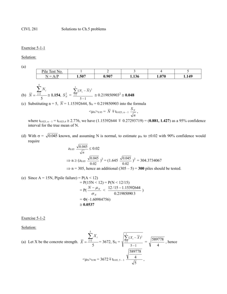
CIVL 281
Solutions to Ch.5 problems
Exercise 5-1-1
Solution:
(a)
Pile Test No.
N = A/P
5
(b) N 
N
i 1
1
2
3
4
5
1.507
0.907
1.136
1.070
1.149
5
i
 1.154,
S N2
=
 (N
i
 N )2
 0.2198509032  0.048
i 1
5
5 1
(c) Substituting n = 5, N = 1.15392644, SN = 0.219850903 into the formula
S
<N>0.95 = N  t0.025, n – 1 N ,
n
where t0.025, n – 1 = t0.025,4  2.776, we have (1.15392644  0.27293719) = (0.881, 1.427) as a 95% confidence
interval for the true mean of N.
(d) With  =
require
0.045 known, and assuming N is normal, to estimate N to 0.02 with 90% confidence would
z0.05
0.045
 0.02
n
 n  (z0.05
0.045 2
) = (1.645
0.02
0.045 2
) = 304.3734067
0.02
 n = 305, hence an additional (305 – 5) = 300 piles should be tested.
(e) Since A = 15N, P(pile failure) = P(A < 12)
= P(15N < 12) = P(N < 12/15)
N  N
12 / 15  1.15392644
= P(
<
)
0.21985090 3
N
= (–1.60984756)
 0.0537
Exercise 5-1-2
Solution:
5
(a) Let X be the concrete strength. X 
X
i 1
5
5
i
= 3672, SX =
( X
<N>0.90 = 3672  t0.05, 5 – 1
i
 X )2
i 1
5 1
589778
4
,
5
=
589778
, hence
4
where t0.05,4  2.131846486, we have (3672  366.0877648) = (3305.91, 4038.09) as a 90% confidence
interval for the true mean of N. Note: our convention is that the subscript p in t p, dof always indicates the tail
area to the right of tp, dof
(b) If the “half-width” of the confidence interval, t/2, 4
589778
4
is only 300 (psi) wide, it implies
5
589778
4
t/2, 4 = 300 / (
) = 1.746996,
5
We need to determine the corresponding . On the other hand, from t-distribution table we have (at 4 d.o.f.)
t 0.1, 4 = 1.533,
t 0.05, 4 = 2.132,
(and t/2, 4 increases as /2 gets smaller in general)
Hence we may use linear interpolation to get an approximate answer: over such a small “x” range (from t =
1.533 to t = 2.132), we treat “y” (i.e. /2) as decreasing linearly, with slope
0.05  0.1
m=
= – 0.083472454
2.132  1.533
Hence, as t goes from 1.533 to 1.746996, /2 should decrease from 0.1 to
/2 = 0.1 + m(1.746996 – 1.533)
= 0.1 – 0.0834724540.213996232 = 0.082137209
  = 20.082137209 = 0.164274419
Hence the confidence level is 1 –  = 1 – 0.164274419  83.6%
Text 5.7
(a) Let xi be the DO recorded on the i-th day. Using the formulas
x
 xi
i 1
 x
n
n
and s 
i 1
i
 x
2
,
n 1
n
where n = 10 is our sample size, we obtain the point estimates for the population mean and standard
deviation:
  x = 2.03 (mg/L), and
  s  0.485 (mg/L)
(b) We are dealing with a normal population with  unknown, which calls for the use of a student-t
distribution; thus a 95% confidence interval for  is formed by
s
xt*
, where
n
where  t* denote the limits between which the t-distribution with (n - 1) degrees of freedom covers an
area of 95%. From tables, t* = t0.975;9 = 2.262, hence, plugging in these numbers and the answers from
(a), we get
[1.68 mg/L, 2.38 mg/L]
as our 95% confidence interval for 
(c) The 95% lower confidence limit for  is obtained as
s
,
x  t 0.95;9
n
where t0.95;9 =1.833 from tables. Using the answers from (a), we obtain 1.75 mg/L as a 95% lower
confidence limit for the true mean DO concentration.
Text 5.10
Assuming population normality, and since n = 9, x = 20 (kips),
(a) A 90% confidence interval for  is formed by the endpoints
x  z*

,
n
where the standard normal curve covers an area of 0.9 from between  z*. Tables (for Z) tell us that z*
 1.645, hence, assuming  = 3 (kips), the confidence limits are
3
.
20  1645
= [20 + 1.645, 20 - 1.645], i.e.
9
[18.36, 21.65] is a 90% confidence interval for the population mean strength (in kips).
.
(b) Let the required sample size be r. A 95% confidence interval would be formed by x  196
equating this to the numbers from part (a)
3
 2165
. 4
 20 + 1.96
r
2
. 3
 r  196
21654
.


196
.

r
 1645
.

9

r
;