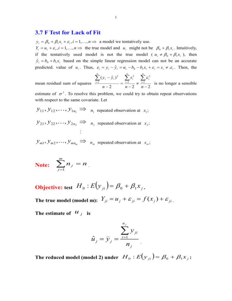
1
3.7 F Test for Lack of Fit
yi   0  1 xi   i , i  1,, n  a model we tentatively use.
Yi  ui   i , i  1,, n  the true model and u i might not be  0  1 xi . Intuitively,
if the tentatively used model is not the true model ( ui   0  1 xi ), then
yˆ i  b0  b1 xi based on the simple linear regression model can not be an accurate
predicted. value of u i . Thus, ei  yi  yˆ i  ui  b0  b1 xi   i  si  . i . Then, the
n
(y
mean residual sum of squares
i 1
i
 yˆ i ) 2
n2
n

s
i 1
n
2
i
n2


i 1
2
i
n2
is no longer a sensible
estimate of  2 . To resolve this problem, we could try to obtain repeat observations
with respect to the same covariate. Let
y11 , y12 , , y1n1 
n1 repeated observation at x1 ;
y 21 , y 22 ,, y 2 n2 
n 2 repeated observation at x2 ;

ym1 , ym 2 , , ymnm 
m
Note:
n
j 1
j
n m repeated observation at x m ;
n.
 
Objective: test H 0 : E y ji   0  1 x j .
The true model (model m):
The estimate of
Y ji  u j   ji  f ( x j )   ji .
u j is
nj
uˆ j  y j 
y
i 1
nj
ji
.
 
The reduced model (model 2) under H 0 : E y ji   0   1 x j :
2
y ji   0  1 x j   ji .
The fitted value of
y ji in reduced model is
ˆj.
yˆ ji  b0  b1 x j  y
yˆ ji  yˆ j
uˆ j  y j
(model 2)
(model m)
y ji
RSS model 2  RSS (model m)
(data)
R S S(m o d eml )
RSS (model m)    y ji  uˆ j     y ji  y j 
nj
m
m
2
j 1 i 1
nj
2
j 1 i 1
2
RSS (model 2)    y ji  yˆ ji     y ji  b0  b1 x j 
nj
m
m
2
j 1 i 1
m
nj
j 1 i 1
nj
  e 2ji
j 1 i 1
 residual sum of squares in simple linear regression
nj
m
m
nj
RSS model 2  RSS model m    (uˆ j  yˆ ji )   ( y j  yˆ j ) 2
2
j 1 i 1
j 1 i 1
m
  n j ( y j  yˆ j ) 2
j 1
Note:
RSS (model m)    y ji  y j 
m
nj
2
j 1 i 1
is called pure error sum of
squares.
m
RSS model 2  RSS model m   n j ( yˆ j  y j ) 2 is called lack of fit
j 1
sum of squares.
3
Note:
Fundamental Equation:
m
nj
 ( y
j 1 i 1
m
nj
m
 yˆ j )   ( y ji  y j )   n j ( y j  yˆ j ) 2 .
2
ji
2
j 1 i 1
j 1
That is
Residual sum of squares (model 2) = Pure error sum of squares
+ Lack of fit sum of squares
m
Let
y
nj
 y
j 1 i 1
n
ji
. The ANOVA table is
Source
df
Due to regression( b1 | b0 )
1
SS
MS
m
m
 n j ( yˆ j  y ) 2
n
j 1
Lack of fit
m-2
m
n
j 1
j
j 1
m
n
( y j  yˆ j ) 2
j 1
j
j
( yˆ j  y ) 2
( y j  yˆ j ) 2
m2
Pure error
n-m
m
nJ
 ( y
j 1 i 1
ji
m
nj
 ( y
 y j )2
j 1 i 1
ji
 y j )2
n p
m
Total (corrected)
nj
 ( y
n-1
j 1 i 1
To test
ji
 y) 2
H 0 : E  y ji    0  1 x j
m
RSS model 2  RSS model m 
F
RSS model m 
nm
n (y
j
j 1
m2 
j
 yˆ j ) 2
m2
m
nj
 ( y
j 1 i 1
ji
 y j )2
nm
In general, we use the following procedure to fit simple regression
4
model when the data contain repeated observations.
1. Fit the model, write down the usual analysis of variance table. Do
not perform an F-test for regression ( H 0 : 1  0 ).
2. Perform the F-test for lack of fit. There are two possibilities.
(a) If significant lack of fit, stop the analysis of the model fitting
and seek ways to improve the model by examining residuals.
(b) If lack of fit test is not significant, carry out an F-test for
regression, obtain confidence interval and so on. The residuals
should still be plotted and examined for peculiarities.
Example:
10
x
i 1
i
X
Y
90
79
66
51
35
81,83
75
68,60,62
60,64
51,53
10
10
10
10
i 1
i 1
i 1
i 1
 629,  y i  657,  xi2  43161,  y i2  44249,  xi y i  43189 .
Thus, total sum of squares:
10
10
 ( yi  y ) 2   yi2  10 y 2  44249  10(65.7) 2  1084.1 .
i 1
i 1
10
S
 b1  XY 
S XX
x y
i 1
10
i
x
i 1
2
i
i
 10 x y

 10 x 2
43189  10 * 62.9 * 65.7
 0.51814
43161  10 * (62.9) 2
 regression sum of squares  b12 S XX  965.65636
 residual sum of squares (reduced model)  1084.1  956.66  118.44
Pure error sum of squares:
X
90: Y1 
2
81  83
 82,  (Y1i  Y1 ) 2  (81  82) 2  (83  82) 2  2 .
2
i 1
79: (75  75) 2  0
3
68  60  62
Y3 
 63.33,  (Y3i  Y3 ) 2  (68  63.33) 2  (60  63.33) 2
3
66:
i 1
 (62  63.33) 2  34.67
5
51: Y4 
2
60  64
 62,  (Y4i  Y4 ) 2  (60  62) 2  (64  62) 2  8.
2
i 1
35: Y5 
2
51  53
 52,  (Y5i  Y5 ) 2  (51  52) 2  (53  52) 2  2
2
i 1
Then, pure error sum of squares=2+0+34.67+8+2=46.67
Lack of fit sum of squares=118.44-46.67=71.77
Source
SS( b1 | b0 )
df
SS
MS
Lack of fit
1
3
965.66
71.77
965.66
23.92
Pure error
5
46.67
9.33
Total (corrected)
F
9
1084.1
23.92
 2.56  f 3,5, 0.05  5.41
9.33
 Not significant!! That is, the simple linear regression is adequate. The standard
F-test for regression can be carried out.