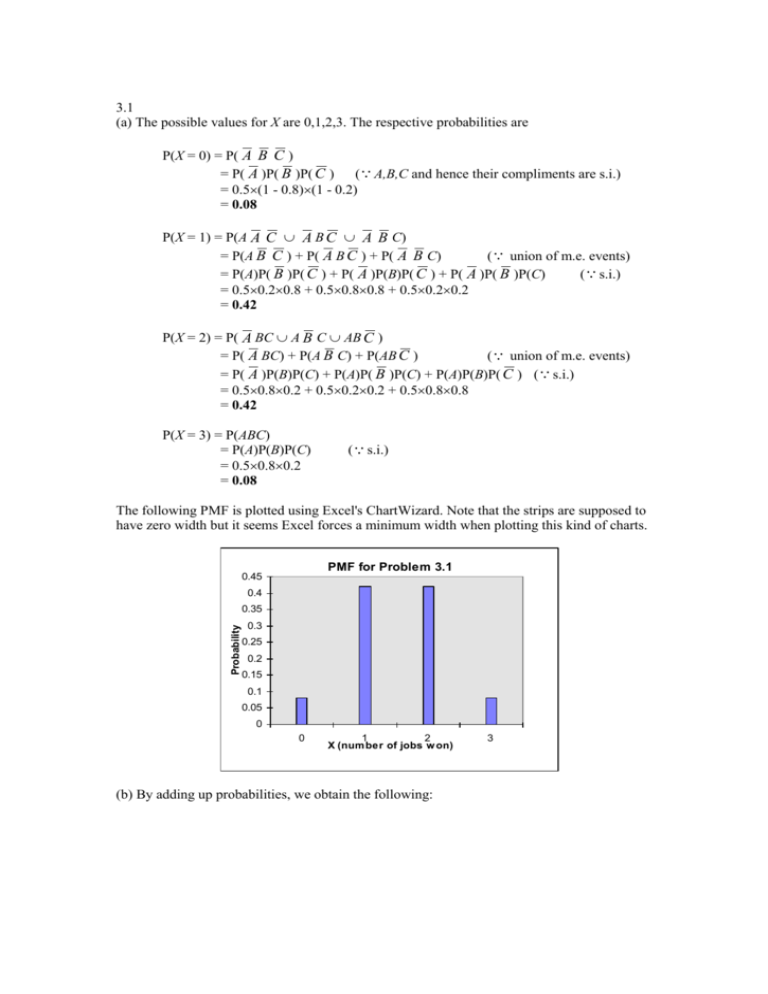
3.1
(a) The possible values for X are 0,1,2,3. The respective probabilities are
P(X = 0) = P( A B C )
= P( A )P( B )P( C ) ( A,B,C and hence their compliments are s.i.)
= 0.5(1 - 0.8)(1 - 0.2)
= 0.08
P(X = 1) = P(A A C  A B C  A B C)
= P(A B C ) + P( A B C ) + P( A B C)
( union of m.e. events)
= P(A)P( B )P( C ) + P( A )P(B)P( C ) + P( A )P( B )P(C)
( s.i.)
= 0.50.20.8 + 0.50.80.8 + 0.50.20.2
= 0.42
P(X = 2) = P( A BC  A B C  AB C )
= P( A BC) + P(A B C) + P(AB C )
( union of m.e. events)
= P( A )P(B)P(C) + P(A)P( B )P(C) + P(A)P(B)P( C ) ( s.i.)
= 0.50.80.2 + 0.50.20.2 + 0.50.80.8
= 0.42
P(X = 3) = P(ABC)
= P(A)P(B)P(C)
= 0.50.80.2
= 0.08
( s.i.)
The following PMF is plotted using Excel's ChartWizard. Note that the strips are supposed to
have zero width but it seems Excel forces a minimum width when plotting this kind of charts.
PMF for Problem 3.1
0.45
0.4
Probability
0.35
0.3
0.25
0.2
0.15
0.1
0.05
0
0
1
2
X (num ber of jobs w on)
(b) By adding up probabilities, we obtain the following:
3
Distribution Function for X (# of jobs won)
FX(x)
0.92 + 0.08 = 1
0.5 + 0.42 = 0.92
1
0.08+0.42 = 0.5
0.5
0.08
0
1
2
3
4
x
(c) P(X  2) = FX(2) = 0.92 (note: FX is right-continuous, i.e. FX(a) = FX(a+)
(d) P(0 < X  2) = FX(2) – FX(0) = 0.92 – 0.08 = 0.84
3.5
Let
R = "Road completed within 15 months";
B = "Bridge completed within 15 months"
P(Project completion within 15 months)
= P(RB)
= P(R)P(B) since R and B are s.i.
So let's first calculate the individual probabilities
P(R) = area of rectangle PDF from t = 12 to t = 15
= (1/6)(15 - 12) = 0.5, while
P(B) = area of triangle PDF from t = 10 to t =15
= (15 - 10)(1/5/2)2 = 0.25
Hence
P(RB) = 0.50.25 = 0.125
3.6
Let Fi denote the event "device fails to detect the i-th existing crack" , where i goes from 1 to
N, N being the total number of cracks.
(a) Given: N = 2. In this case,
P(two cracks both go undetected)
= P(F1 F2)
= P(F1)P(F2)
= 0.20.2
= 0.04
(b)
Let FAC denote "device fails to detect any crack at all”.
If there is indeed no crack, the device certainly will not detect anything, i.e.
P(FAC | N = 0) =1;
while we’re given P(successful detection | N = 1) = 0.8, hence
P(FAC | N = 1) = 1 – 0.8 = 0.2, and
P(FAC | N = 2) = 0.04
as calculated in part(a). Note that N is a random variable in this case, hence by the total
probability theorem,
P(FAC)
= P(FAC | N = 0)P(N = 0) + P(FAC | N = 1)P(N = 1) + P(FAC | N = 2)P(N = 2)
= 10.3 + 0.20.6 + 0.040.1
= 0.424
(c) The mean of N is  N 
 nP( N  n)
n  0 ,1, 2
= 00.3 + 10.6 + 20.1 = 0.8
The variance of N is  N2 
 n   
n  0 ,1, 2
2
N
P ( N  n)
= (0 - 0.8)20.3 + (1 - 0.8)20.6 + (2 - 0.8)20.1 = 0.36
The coefficient of variation of N is  N 
N
N
=
0.36
= 0.75
0.8
(d) By Bayes' theorem, P(N = 0 | FAC)
= P(FAC | N = 0)P(N = 0)  P(FAC)
= 10.3  0.424  0.708
Picture for parts (b) and (d) (not to scale; just to provide a qualitative idea):
N=1
N=0 N=2
Failure
to
detect
any
crack
3.17
Given: M is Gaussian with mean 50 and standard deviation 0.2*50, i.e. M ~ N(50, 10)
(a) Let O denote the clamped end. If a load of 3 kips is applied at the free end, it gives a
moment about O,
M0 = (3 kips)(10 ft) = 30 kip-ft
With pf denoting the beam failure probability,
pf = P(M < M0)
= P(
M  50 30  50

)
10
10
= P(Z < -2)  0.023
(b) The uniform load gives a moment about O
10
10
x 0
x 0
 dM   xdF
Mu =
10
=
 x(0.5)dx
x 0
= 0.5(10)2/2 (kip-ft)
= 25 kip-ft
hence
pf = P(M < M0 + Mu)
= P(
M  50 30  25  50

)
10
10
= P(Z < -0.5)  0.006
(c) In the case of the combined load (30 + 25) = 55 kip-ft
pf = P(M < 55)
= P(
M  50 55  50

)
10
10
= P(Z < -0.5)  0.3085
(d) Given event: M > 30, thus the conditional probability of surviving the combined load is
P(M > 55 | M > 30)
= P(M > 55 and M > 30) / P(M > 30)
= P(M > 55) / P(M > 30)
= P(
M  50 55  50
M  50 30  50


) / P(
)
10
10
10
10
= [1 - P(Z < 0.5)] / [1 - P(Z < -2)]
 0.308538 / 0.308538  0.316
(e) For a uniform load of w (kip/ft), the resultant Mu = 50w (kip-ft). Hence if we want to
enforce
P(M > Mu) = 0.995, i.e.
P(M > 50w) = 0.995
M  50 50w  50

) = 0.995,
10
10
50w  50
 P( Z 
) = 0.995, i.e.
10
50w  50
P(Z 
) = 0.005
10
 P(
comparing to what a table (or Excel) says:
P(Z  - 2.575835) = 0.005,
we must have
50w  50
= - 2.575835
10
 w  0.485 kip/ft (or less)
3.19
Given information:
X = 30
P(X  40) = 0.9
(a) Rewriting (ii) in a standardized form,
P(
X  30
X

40  30
X
(i)
(ii)
)  0.9
(iii)
If we assume X is Gaussian (i.e. normal), then (X - 30) / X is a standard normal variate,
hence (iii) becomes
40  30
P( Z 
)  0.9
(iv)
X
but, from Table A.1 of the text, P( Z  1285
. )  0.9 . Comparing this to (iii), we must have
40  30
X
 1285
.
, hence
X = 10 / 1.285  7.78,
hence
P(X < 50) = P (
X  30

50  30
)
7.782101167

0  30
)
7.782101167
X
= P(Z < 2.57)
 0.995
(b) Based on the normality assumption,
P(X < 0) = P (
X  30
X
= P(Z < - 3.855)
 1- 0.99994
 0.00006
The normality assumption leads to a finite probability for a physically impossible event,
so it's no all that reasonable.
(c) Now let's assume X is log-normal (i.e. ln(X) is normal) with the same expected value and
variance as in (a). These allow us to determine its parameters
 
  ln(1   X  )
 X 
2
2
= ln [1 + (7.782101167 / 30)2]
= 0.0651228285
 0.065
while
1
2
  ln  X   2
= ln (30) - 0.0651228285 / 2
= 3.368635968
 3.37
Hence
P(X < 50) = P(ln X < ln 50)
= P(
ln X  

= P(Z < 2.129)

ln 50  3.368635968
)
0.0651228285
 0.983
X 
 = 0.0672901095 and hence  
(or 0.982 if you had used approximated   
 X 
2
2
3.367552327)
(a) and (b) results are quite close; the percentage difference being only about 1%.
3.20
Let T be the time (in months) between breakdowns. Given: T is log-normal, with
T  6,  T  15
.
 T 
15
.
 0.25
6
which is small, hence we may use the approximation
 2  T 2  0.0625,
and hence
  ln T 
2
2
 ln 6 
0.0625
 1760509469
.
2
 and  are the respective variance and mean of ln(T), which is normally distributed.
2
(a) Suppose a piece of equipment is checked every T0 months. The requirement that there is
"at least a 90% probability that a piece of equipment will be operational at any time" means
we want "10% (or less) probability that the equipment breaks down before being maintenance
is performed", hence we require
P(T  T0) = 0.1,
or
P(
ln T  


ln T0  

) = 0.1
ln T0  1760509469
.
) = 0.1,
0.25
ln T0  1760509469
.

= -1(0.1)  -1.285
0.25
P(Z 
T0 = 4.217571418
 4.22 (months)
 Each piece of equipment should be checked at least every 4.22 months to ensure a 90%
chance of being operational.
(b) "At maintenance time, the equipment still hasn't had a breakdown" means "T > 4.22". To
be operational for at least one more month without any maintenance means "T > 5.22". Hence
the desired probability is
P(T > 5.22| T > 4.22)
= P(T > 5.22 and T > 4.22) / P(T > 4.22)
= P(T > 5.22) / P(T > 4.22)
where
P(T > 5.22)
= P(
ln T  


ln(522
. )

)
= P( Z 
ln(5.217571418)  1760509469
.
)
0.25
= P(Z > -0.4339) = P(Z < 0.4339)  0.668
P(T > 4.22) = 0.9,
P(T > 5.22 | T > 4.22)
= 0.668 / 0.9  0.742
and
hence
3.21
(a) Let N be the number of rainstorms in a year. From the given PMF of N, we can calculate
its mean and variance as follows:
E(N)  <n> =
 n  f (n) = 0*0.3 + 1*0.4 + 2*0.2 + 3*0.1
all
= 1.1
Var(N) =
 ( n   n )
2
 f ( n)
all
= (0 - 1.1)20.3 + (1 - 1.1)20.4 + (2 - 1.1)20.2 + (3 - 1.1)20.1
= 0.89
(b) let R be the maximum runoff rate (in ft3 / s) in a storm; we're given that R is log-normal
with median rm = 7, and COV = 0.15. From formulas 3.32(a) and 3.33,
 = ln(rm) = ln(7);
  0.15
hence
P(flooding during a rainstorm)
= P(R > 8)
= P(
ln R  


ln 8  

)
= P(Z > 0.890209)
= 1 - P(Z  0.890209)
 1 - 0.81332
= 0.187
(c) From part (b), we have the probability of flooding given one rainstorm is 0.187 (call it p).
If there is zero or one storm in a year, the respective probabilities of flooding are zero and p,
obviously. Furthermore, with Fi denoting "flooding occurs during the i-th storm",
P(flooding in a year | 2 rainstorms in that year)
= P(F1  F2)
= P(F1) + P(F2) - P(F1 F2)
= p + p - pp
= p(2 - p)
whereas
P(flooding in a year | 3 rainstorms in that year)
= 1 - P(no flooding at all)
= 1 - P( F1  F2  F3 )
= 1 - (1 - p)3
Hence we may apply the theorem of total probability to calculate
P(flooding in a year)
=

P(flooding | n rainstorms in a year)P(n rainstorms in that year)
n 0 ,1, 2 , 3
= 0*0.3 + p*0.4 + p(2 - p)*0.2 + [1 - (1 - p)3]*0.1
 0.189
(where p = 0.186676723 from (b))
3.27
Since the rainfall return period is 10 years, the probability of sewer flooding is
1
= 0.1 (probability per year)
10 years
(a) Suppose the first flooding occurs in the T-th year, then T follows a geometric distribution
with parameter p = 0.1 , hence
P(first flooding in the third year)
= P(T = 3)
= p (1 - p)3 - 1
= 0.1 (0.9)2
= 0.081
(b) Let Fi denote "there is flooding during the i-th year"
P(any flooding within the first 3 years)
= 1 - P(no flooding at all within the first 3 years)
= 1 - P( F1  F2  F3 )
= 1 - P( F1 )P( F2 )P( F3 )
= 1 - (1 - p)3
= 1 - 0.93
= 0.271
(assuming s.i.)
(c) Let X be the total number of years with flooding among the first five years, then X follows
a binomial distribution with p = 0.1 and n = 5. Hence
P(flooding in 3 of the first 5 years)
= P(X = 3)
=
5!
(01
. ) 3 (1  01
. ) 5 3
3!(5  3)!
= 0.0081
(d) Let Y be the total number of floods within 3 years, then Y follows a binomial distribution
with p = 0.1 and n = 3. Hence
P(one flood within 3 years)
= P(Y = 1)
= 3p(1 - p)2
= 0.243
Note: in Excel, one can get the binomial probability b(x; n,p) by typing the following:
=binomdist(x,n,p,false)
For example, in any empty cell, typing in (hit enter after typing it)
=binomdist(3,5,0.1,false)
gets you the answer (0.0081) in part (c).