Random and Mixed-Effects Model
Model II (Random Factor Levels) for Two-factor Studies
What we have considered:
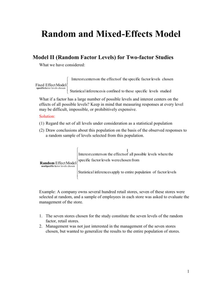
 Interest centers on the effects of the specific factor levels chosen

Fixed Effect Model
specificfactor levels chosen
 Statistica l inferences is confined to these specific levels studied

What if a factor has a large number of possible levels and interest centers on the
effects of all possible levels? Keep in mind that measuring responses at every level
may be difficult, impossible, or prohibitively expensive.
Solution:
(1) Regard the set of all levels under consideration as a statistical population
(2) Draw conclusions about this population on the basis of the observed responses to
a random sample of levels selected from this population.

I
Interest centers on the effects of all possible levels where the

specific factor levels were chosen from
Random Effect Model
nonSpecific factor levels chosen

Statistica l inferences apply to entire population of factor levels


Example: A company owns several hundred retail stores, seven of these stores were
selected at random, and a sample of employees in each store was asked to evaluate the
management of the store.
1. The seven stores chosen for the study constitute the seven levels of the random
factor, retail stores.
2. Management was not just interested in the management of the seven stores
chosen, but wanted to generalize the results to the entire population of stores.
1
One-way random effects model
 i    i
Yij   i   ij
i=1 ,r ;
(1)
(cell means model)
j=1 ,n
Yij    i  ij
(2)
(factor effect model)
i=1 ,r ; j=1 ,n
where:
ui = the effect of the i-th randomly selected treatment, are independent N(0, 2 )
ij =random error, are independent N(0,  2 )
i and ij are mutually independent
----------------------------------------------------------------------------------------------------= the overall mean expected response.
i = the effect of the i-th randomly selected treatment, are independent N(0,  2 )
i and ij are mutually independent
2
Questions of Interest
(1) estimation of 
(2) estimation of 2
(3) estimation of 2
(4) estimation of 2 /( 2+ 2 )
(5) H0 : 2  0
H1 : 2  0
Table 10.1 ANOVA Table: one-way random effect model with equal replication
Source of Variation Degree of
Freedom
Treatments
a-1
Error
a(n-1)
Sum of
Mean
Squares
Square
a
a Y2 Y2
n  (Y i.  Y .. ) 2   i.  ..
n
an
i 1
i 1
a
MSTreatment
Fo
Fo 
MS Treatment
MS E
n
  (Yij  Y i. ) 2
MSE
i 1 j 1
2
a n
2
2 Y..
(
Y

Y
)

Y

  ij ..   ij an
i 1 j 1
i 1 j 1
a
Total
an-1
n
The expected values of these mean squares are known as
E(MS E )   2 ,
E(MSTreatment )   2  n2
3
Estimation of 
ˆ  Y..
2
2
σ 2 nσμ  σ
V(Y.. ) 


r
rn
rn
σμ2
s 2{Y..} 
MSTreatment
rn
The confidence limits for : Y..  t1 α/2,r 1s{Y..}
Estimation of 2 /( 2+ 2 )
MSTreatment /(n2  2 )
MSE / 2
P(F / 2,r 1,r (n 1) 
P (L 
2
2
Where
~ Fr 1,r (n 1)
MSTreatment
2
 F1  / 2,r 1,r (n 1) )  1  
MSE
(n2  2 )
 U)  1  
L
1 MSTreatments
1
(
 1),
n
MSE
F1  / 2 , r  1, r (n  1)
U
1 MSTreatments
1
(
 1),
n
MSE
F / 2 , r  1, r (n  1)
L
2
U
 2  2
L  1   
1 U
4
Example: Apex enterprises studied
personnel officer evaluation ratings of
potential employees. Five of the company’s
personnel officers were randomly selected,
and four job applicants were randomly
assigned to each of the five officers. Thus
each officer rated four job applicants.
Obs
y
officer
Candidate
1
76
1
1
2
65
1
2
3
85
1
3
4
74
1
4
5
59
2
1
.
SAS CODE:
data apex;
infile 'c:\stat231B06\ch25ta01.txt';
input y officer candidate;
run;
proc glm;
class officer;
model y=officer;
/*because the five officers are perceived as a random sample from a */
/*very large "population" of officers, we refer to the factor officers*/
/*as a random factor*/
random officer;
run;
/*To construct confidence intervals for functions of sigma^2,etc.,*/
/*and carry out additional analyses, we use SAS proc mixed. Note that*/
/*the 'method'option can be used to specify the estimation method */
/*[ml=maximum likelihood, reml=residul(restricted)maximum likelihood),*/
/*miqvue0=minimum variance quadratic unbiased estimates. for the */
/*covariance parameters*/
proc mixed method =reml asycov cl covtest
alpha=.1;
class officer;
/*estimate the mean rating of all personnel officers with a 90% *
/*confidence interval*/
model y= / cl alpha=.1;
random officer;
run;
data ratio;
/*use text equation 25.18*/
n=4;
r=5;
mstr=394.925;
mse=73.28333;
fl=finv(1-0.1, r-1, r*(n-1));
fu=finv(0.1, r-1, r*(n-1));
l=1/n*((mstr/mse)*(1/fl)-1);
u=1/n*((mstr/mse)*(1/fu)-1);
lstar=l/(l+1);
ustar=u/(u+1);
proc print data=ratio;
var l u lstar ustar;
run;
5
SAS OUTPUT:
The GLM Procedure
Dependent Variable: y
DF
Sum of
Squares
Mean Square
F Value
Pr > F
Model
4
1579.700000
394.925000
5.39
0.0068
Error
15
1099.250000
73.283333
Corrected Total
19
2678.950000
Source
R-Square
Coeff Var
Root MSE
y Mean
0.589671
11.98120
8.560569
71.45000
Source
DF
Type I SS
Mean Square
F Value
Pr > F
officer
4
1579.700000
394.925000
5.39
0.0068
Source
DF
Type III SS
Mean Square
F Value
Pr > F
officer
4
1579.700000
394.925000
5.39
0.006
We conclude that the means for officers in the population (of officers) are not all equal
because p-value=0.006.
Solution for Fixed Effects
Effect
Intercept
Estimate
Standard
Error
DF
t Value
Pr > |t|
Alpha
Lower
Upper
71.4500
4.4437
4
16.08
<.0001
0.1
61.9768
80.9232
We estimate the mean rating (..) of all personnel officers with a 90% confidence
intervals. This is accomplished by the “method y=/cl alpha=.1;” statement. From the
Solution for Fixed effects table, the estimate is ˆ  71.45 and the confidence limit is
between 61.98 and 80.92
The Mixed Procedure
Covariance Parameter Estimates
Cov Parm
Estimate
Standard
Error
Z
Value
Pr Z
Alpha
Lower
Upper
officer
Residual
80.4104
73.2833
70.1333
26.7593
1.15
2.74
0.1258
0.0031
0.1
0.1
29.5215
43.9774
865.42
151.39
Asymptotic Covariance Matrix of Estimates
Row
CovP1
CovP2
1
Cov Parm
officer
4918.68
-179.01
2
Residual
-179.01
716.06
to estimate sigma^2 with a 90% confidence interval, we use proc mixed and requested
that the asymptotic covariance matrix of the covariance parameters be displayed and that
90% confidence limits be computed to estimate the parameters (asycov, cl, covtest
alpha=.1;). The covtest option produces asymptotic standard errors and Wald Z-test for
the covariance parameter estimates. The 90% confidence interval is calculated between
43.98 and 151.39.
6
Obs
1
l
0.32052
u
4.96436
lstar
0.24272
ustar
0.83234
An estimate of 2 is given by MSE=73.28 (see the first output). The lower and upper limits for
2
2   2
is between 24.272 and 0.83234
Two or more random effects (Model II)
Suppose both factors A and B are random factors, the two-way complete model with
random effects is
Yijk  ..  i   j  ()ij  ijk
i=1 ,a
j=1 ,b
k=1,2 . . . n
..= the overall mean expected response.
i = the effect of the i-th randomly selected treatment, are independent N(0,  2 )
 j = the effect of the j-th randomly selected treatment, are independent N(0, 2 )
2
 ij = the effect of the ij-th randomly selected interaction, are independent N(0,  
)
ijk =random error, are independent N(0,  2 )
i ,  j ,  ij and ijk are pairwise independent
As in a two-way complete model with fixed effects, SSTotal= SSA +SSB +SSAB +SSE
and the calculation for each term is the same.
Model II ANOVA table
Source of Degree of Sum of
Mean
Expected
Variation
Square
MS
Freedom Squares
Fo
7
Factor A
a-1
SSA
MSA 
SS A
(a  1)
Factor B
b-1
SSB
MSB 
SS B
(b  1)
AB
(a-1)(b-1)
E(MSA )
σ
2
 nσ 2 β
 bnσ 2
E(MSB )
σ
2
 nσ 2 β
 anσ2
SSAB
MSAB 
E(MSAB )
SS AB
2
( a  1)(b  1)  σ 2  nσ αβ
MSE 
SS E
ab(n  1)
Fo 
MS A
MS AB
Fo 
MS B
MS AB
Fo 
MS AB
MS E
interaction
Error
ab(n-1)
SSE
Total
abn-1
SSTotal
E(MS E )   2
Hypothesis testing:
2
H0 : 
 0 (no interaction)
2
H1 : 
0
Reject H0 if Fo 
MS AB
>F1-, (a-1)(b-1),ab(n-1)
MS E
When there is no interaction, we can test
H 0 : 2  0
H1 : 2  0
Reject H0 if Fo 
MS A
>F1-, (a-1),(a-1)(b-1)
MS AB
(Note the denominator is not MSE)
We can also test
H 0 : 2  0
H1 : 2  0
Reject H0 if Fo 
MS B
>F, (b-1),(a-1)(b-1)
MS AB
Mixed Models (Model III)
When a model has both fixed effects and random effects, it is called a mixed model. If a
factor is random, its interactions with any other factor will be regarded as random effects.
8
Yijk  ..  i   j  ()ij  ijk
i=1 ,a
j=1 ,b
k=1,2 . . . n
..= the overall mean expected response.
i = the effect of the i-th fixed effect , ai1 i  0
 j = the effect of the j-th randomly selected treatment, are independent N(0, 2 )
 ij = the effect of the ij-th randomly selected interaction, are independent
N(0,
a 1 2
 ) , subject to the restrictions:  ai1 ij  0
a
ijk =random error, are independent N(0,  2 )
 j ,  ij and ijk are pairwise independent
Source of Degree of
Sum of
Mean
Expected
Variation
Squares
Square
MS
Freedom
Fo
E(MSA )
Factor A
a-1
Factor B
AB
b-1
(a-1)(b-1)
SSA
SS A
MSA 
(a  1)
SS B
(b  1)
SSB
MSB 
SSAB
MSAB 
MSE 
a
 αi
2
2
 σ 2  nσ αβ
 bn i 1
a 1
E(MS B )
σ
2
 anσ β2
E(MSAB )
SS AB
( a  1)(b  1)  σ 2  nσ 2 β
Fo 
MS A
MS AB
Fo 
MS B
MS E
Fo 
MS AB
MS E
interaction
Error
ab(n-1)
SSE
Total
abn-1
SSTotal
SS E
ab(n  1)
E(MS E )   2
Hypothesis testing:
9
H 0 :  2  0 (no interaction)
H1 :  2  0
Reject H0 if Fo 
MS AB
>F1-, (a-1)(b-1),ab(n-1)
MS E
When there is no interaction, we can test
H 0 :  2  0
H1 :  2  0
Reject H0 if Fo 
MS A
>F1-, (a-1),(a-1)(b-1)
MS AB
(Note the denominator is not MSE)
We can also test
H 0 : 2  0
H1 : 2  0
Reject H0 if Fo 
MS B
>F1-, (b-1),ab(n-1)
MS E
10