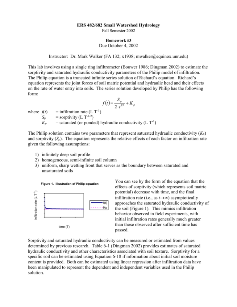
ERS 482/682 Small Watershed Hydrology
Fall Semester 2002
Homework #3
Due October 4, 2002
Instructor: Dr. Mark Walker (FA 132; x1938; mwalker@equinox.unr.edu)
This lab involves using a single ring infiltrometer (Bouwer 1986; Dingman 2002) to estimate the
sorptivity and saturated hydraulic conductivity parameters of the Philip model of infiltration.
The Philip equation is a truncated infinite series solution of Richard’s equation. Richard’s
equation represents the joint forces of soil matric potential and hydraulic head and their effects
on the rate of water entry into soils. The series solution developed by Philip has the following
form:
Sp
f t  
 Kp
2  t1 2
where f(t)
= infiltration rate (L T-1)
Sp
= sorptivity (L T-1/2)
Kp
= saturated (or ponded) hydraulic conductivity (L T-1)
The Philip solution contains two parameters that represent saturated hydraulic conductivity (Kh)
and sorptivity (Sp). The equation represents the relative effects of each factor on infiltration rate
given the following assumptions:
1) infinitely deep soil profile
2) homogeneous, semi-infinite soil column
3) uniform, sharp wetting front that serves as the boundary between saturated and
unsaturated soils
infiltration rate (L T-1 )
Figure 1. Illustration of Philip equation
30
25
20
15
10
5
0
f(t)
Kp
0
200
time (T)
400
You can see by the form of the equation that the
effects of sorptivity (which represents soil matric
potential) decrease with time, and the final
infiltration rate (i.e., as t) asymptotically
approaches the saturated hydraulic conductivity of
the soil (Figure 1). This mimics infiltration
behavior observed in field experiments, with
initial infiltration rates generally much greater
than those observed after sufficient time has
passed.
Sorptivity and saturated hydraulic conductivity can be measured or estimated from values
determined by previous research. Table 6-1 (Dingman 2002) provides estimates of saturated
hydraulic conductivity and other characteristics associated with soil texture. Sorptivity for a
specific soil can be estimated using Equation 6-18 if information about initial soil moisture
content is provided. Both can be estimated using linear regression after infiltration data have
been manipulated to represent the dependent and independent variables used in the Philip
solution.
ERS 482/682 (Fall 2002)
Homework #3
In this laboratory, you will work in groups of two and obtain two types of measurements to
characterize the change in infiltration rates with time under ponded conditions. The first will be
an estimate of initial soil water content (0). The second will be a time series of volumes of
water added to a single-ring infiltrometer. You will use this information to compare the
differences between infiltration estimates made using 1) the changes in infiltration rates with
time observed; 2) parameter estimations provided in Table 6-1 and Equation 6-18; and 3) leastsquares regression.
Procedures:
1. Obtain starting soil moisture data (0; see Equation 6-6 and use Equation[24] in Gardner
1986).
2. Carry out infiltration experiments with single ring infiltrometers as described by Bouwer
(1986). You will apply the following modified method:
a. Drive rings into soil to recommended depth.
b. Add water to depth of 1” (interior) using a graduated cylinder. Maintain the water
level at 1” depth. Record the volume increments added to maintain this water level,
and the times at which the water is added. Continue until the infiltration rate
approximately stabilizes.
Products Expected:
Note: Each group should turn in ONE report; be sure to write the names of all of your group
members on your report!
1. A graph of infiltration rate as a function of time with four series of infiltration rates:
a) infiltration rates you observed (dots)
b) corrected infiltration rates based on the critical pressure head hcr and corresponding
adjustments according to Figure 32-4 in Bouwer (1986) (squares)
c) infiltration rates estimated using values from Table 6-1 and Equation 6-18 (line with
no dots)
d) infiltration rates determined with parameters estimated from the observed data with
the least squares approach in Box 6-2 (Dingman 2002; see Equations 6B2-9, 6B2-8,
and 6-31a)) (heavy line)
2. Your estimate of the starting soil moisture content (0), critical pressure head hcr, and the
adjustment factor you used to correct the observed infiltration rates
3. Your estimates of saturation hydraulic conductivity (Kp) in cm hr-1 (for series a, b, and c,
estimate Kp from your plots; for series d use Equation 6B2-8)
4. Your estimates of sorptivity (Sp) in cm hr-1/2 using Equation 6-18 for series c, and Equation
6B-9 for series d
5. Calculate the correlation coefficient r for series c and series d, using series a as the observed
data; provide a short discussion of the strength of the relationships and observed differences
or similarities between the four approaches.
6. A comparison of your results from all four approaches with the observed data obtained from
the same experiment carried out on other plots by other groups in this lab, including 0 and
your estimates of Kp and Sp for each group’s data (estimate Kp from their observed data and
2
ERS 482/682 (Fall 2002)
Homework #3
3
use Equation 6-18 to estimate Sp); do not adjust the observed data for the other groups as you
did for Item 1b.
7. A discussion of the differences and similarities between results obtained for each group;
discuss how experimental technique and soil characteristics might have led to the differences
in results.
Useful information:
Soil fraction composition:
5% fine gravel
65% sand
14% silt
16% clay
Using a spreadsheet to estimate Kp and Sp using least squares approach with the Philip equation:
 Put your observed data into a spreadsheet (one column for time t, one column for
calculated infiltration rate based on observation at time t); be sure to use appropriate
units!
 Adjust t so that it represents time from ponding
f t   1
1
 Create columns to corresponding to f t i , 1 2i , , and 1 2 ; calculate
ti
ti
ti


 f t     1   1 
 f t i ,   1 2i ,   ,   1 2 
 t i   t i   t i 
Calculate Sp using Equation 6B2-9 (Dingman 2002)
Calculate Kp using Equation 6B2-8; note there is an error in the formulation in Dingman
 1 
2 f ti   S p   1 2 
 ti 
(2002); the equation should be K p 
2N
The correlation coefficient provides a measure of how much the variability of the observed data
is correlated with the variability of the estimated data. To calculate the correlation coefficient r,
you can use the CORREL function in Excel:
Syntax
CORREL(array1,array2)
Array1 is a cell range of values.
put the y (estimated) values here
Array2 is a second cell range of values
put the x (original observed) values here
ERS 482/682 (Fall 2002)
Homework #3
4
References:
Bouwer H. 1986. pp 825-843 in Methods of Soil Analysis – Part I: Physical and Mineralogical
Methods. Madison (WI): American Society of Agronomy – Soil Science Society of America.
Dingman L. 2002. Physical Hydrology (2nd ed.). Upper Saddle River (NJ):Prentice-Hall.
Gardner W. 1986. pp 493-544 in Methods of Soil Analysis – Part I: Physical and Mineralogical
Methods. Madison (WI): American Society of Agronomy – Soil Science Society of America.