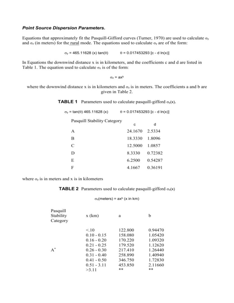
Point Source Dispersion Parameters.
Equations that approximately fit the Pasquill-Gifford curves (Turner, 1970) are used to calculate y
and z (in meters) for the rural mode. The equations used to calculate y are of the form:
y = 465.11628 (x) tan()
 = 0.017453293 [c - d ln(x)]
In Equations the downwind distance x is in kilometers, and the coefficients c and d are listed in
Table 1. The equation used to calculate z is of the form:
z = axb
where the downwind distance x is in kilometers and z is in meters. The coefficients a and b are
given in Table 2.
TABLE 1 Parameters used to calculate pasquill-gifford y(x).
y = tan() 465.11628 (x)
 = 0.017453293 [c - d ln(x)]
Pasquill Stability Category
c
d
A
24.1670
2.5334
B
18.3330
1.8096
C
12.5000
1.0857
D
8.3330
0.72382
E
6.2500
0.54287
F
4.1667
0.36191
where y is in meters and x is in kilometers
TABLE 2 Parameters used to calculate pasquill-gifford z(x)
z(meters) = axb (x in km)
Pasquill
Stability
Category
x (km)
a
b
A*
<.10
0.10 - 0.15
0.16 - 0.20
0.21 - 0.25
0.26 - 0.30
0.31 - 0.40
0.41 - 0.50
0.51 - 3.11
>3.11
122.800
158.080
170.220
179.520
217.410
258.890
346.750
453.850
**
0.94470
1.05420
1.09320
1.12620
1.26440
1.40940
1.72830
2.11660
**
B*
<.20
0.21 - 0.40
>0.40
90.673
98.483
109.300
0.93198
0.98332
1.09710
C*
All
61.141
0.91465
D
.30
0.31 - 1.00
1.01 - 3.00
3.01 - 10.00
10.01 - 30.00
>30.00
34.459
32.093
32.093
33.504
36.650
44.053
0.86974
0.81066
0.64403
0.60486
0.56589
0.51179
E
<.10
0.10 - 0.30
0.31 - 1.00
1.01 - 2.00
2.01 - 4.00
4.01 - 10.00
10.01 - 20.00
20.01 - 40.00
>40.00
24.260
23.331
21.628
21.628
22.534
24.703
26.970
35.420
47.618
0.83660
0.81956
0.75660
0.63077
0.57154
0.50527
0.46713
0.37615
0.29592
F
<.20
0.21 - 0.70
0.71 - 1.00
1.01 - 2.00
2.01 - 3.00
3.01 - 7.00
7.01 - 15.00
15.01 - 30.00
30.01 - 60.00
>60.00
15.209
14.457
13.953
13.953
14.823
16.187
17.836
22.651
27.074
34.219
0.81558
0.78407
0.68465
0.63227
0.54503
0.46490
0.41507
0.32681
0.27436
0.21716
* If the calculated value of z exceed 5000 m, z is set to 5000 m.
** z is equal to 5000 m.
Tables 3 and 4 show the equations used to determine y and z for the urban option. These
expressions were determined by Briggs as reported by Gifford (1976) and represent a best fit to
urban vertical diffusion data reported by McElroy and Pooler (1968). While the Briggs functions
are assumed to be valid for downwind distances less than 100m, the user is cautioned that
concentrations at receptors less than 100m from a source may be suspect.
TABLE 3
(x is in meters)
Pasquill Stability
Category
y(meters)*
A
0.32 x (1.0 + 0.0004 x)-1/2
B
0.32 x (1.0 + 0.0004 x)-1/2
C
0.22 x (1.0 + 0.0004 x)-1/2
D
0.16 x (1.0 + 0.0004 x)-1/2
E
0.11 x (1.0 + 0.0004 x)-1/2
F
0.11 x (1.0 + 0.0004 x)-1/2
TABLE 4
(x is in meters)
Pasquill Stability
Category
z(meters)*
A
0.24 x (1.0 + 0.001 x)1/2
B
0.24 x (1.0 + 0.001 x)1/2
C
0.20 x
D
0.14 x (1.0 + 0.0003 x)-1/2
E
0.08 x (1.0 + 0.0015 x)-1/2
F
0.08 x (1.0 + 0.0015 x)-1/2