Chapter 3, Random Variables and Probability Distributions
3.1 Random variables
(1) An example:
- How to calculate the average grade of a student?
- Use random variable, the example: what is the grades of a student
marks
comments
r. v. (X)
F
failed
0
D, C
passed
1
B
good
2
A
excellent
3
(2) Definition:
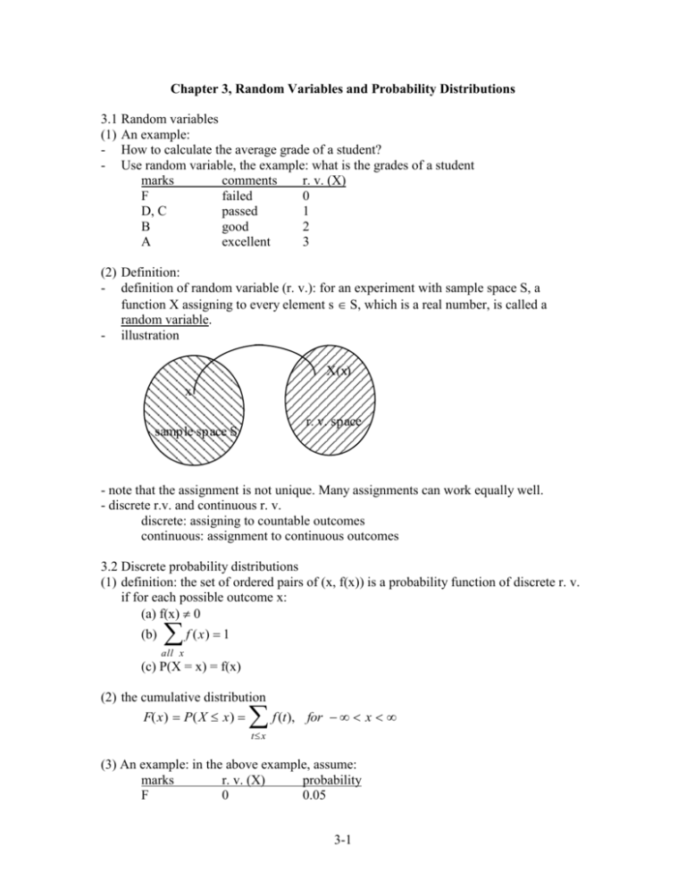
- definition of random variable (r. v.): for an experiment with sample space S, a
function X assigning to every element s  S, which is a real number, is called a
random variable.
- illustration
X(x)
x
r. v. space
sample space S
- note that the assignment is not unique. Many assignments can work equally well.
- discrete r.v. and continuous r. v.
discrete: assigning to countable outcomes
continuous: assignment to continuous outcomes
3.2 Discrete probability distributions
(1) definition: the set of ordered pairs of (x, f(x)) is a probability function of discrete r. v.
if for each possible outcome x:
(a) f(x)  0
f (x)  1
(b)

all x
(c) P(X = x) = f(x)
(2) the cumulative distribution
F(x)  P(X  x) 
f (t), for    x  

t x
(3) An example: in the above example, assume:
marks
r. v. (X)
probability
F
0
0.05
3-1
D, C
B
A
1
2
3
0.25
0.5
0.2
then:
f(3) = P(X = 3) = 0.2
F(X) = P(X  1) = 0.25 + 0.5 + 0.2 = 0.95
another way to calculate:
F(X  1) = 1 - P(X = 0) = 1 - 0.05 = 0.95
3.3 Continuous probability distribution
(1) When X is a continuous r. v., f(x) is a probability density function, which satisfy:
(a) f(x)  0, for all x
(b)

 f (x)dx  1
b
(c) P(a  X  b)   f (x)dx
a
(2) The cumulative distribution
F(x)  P(X  x)  
x

f (t)dt , for - < x < 
- note:
P(a < X < b) = F(b) - F(a)
dF(x)
f (x)  dx
F(x) = 0
3.4 Empirical distributions
(1) Empirical distribution is a probability model that often used in data analysis
(2) How to obtain empirical distribution: the example
 the data (number of hours of exercise per week of the 12 students)
 the stem-leaf plot
stems
00
02
04
06
08
10


leaves
0,0
4, 4, 4, 5, 5
6, 7
8
0, 0
frequency
2
0
5
2
1
2
the histogram
estimating the probability distribution
3-2
relative frequency
1/6
0
5/12
1/6
1/12
1/6
3.5 Joint probability distributions
(1) The example: what is the probability of picking a student who is a female and
exercises 5 hours per week?
(2) The definition of joint probability (for discrete r. v.): the function f(x, y) is a joint
probability distribution of the discrete r. v. X and Y if
(a) f(x, y)  0, for all (x, y)
(b)  f ( x, y )  1
x
y
(c) P(X = x, Y = y) = f(x, y)
-
For any region A in the xy plane,
P[(X,Y) A]    f (x,y)
A
(3) The example:
- the definition of the r. v.
X2:
0 - Male
1 - Female
X4:
0 - 0 hours
1 - 4 hours
2 - 5 hours
3 - 6 hours
4 - 7 hours
5 - 8 hours
6 - 10 hours
- the joint probability distribution
X4 \ X2
0 (M)
0 (0)
1/12
1 (4)
3/12
2 (5)
0
3 (6)
1/12
4 (7)
0
5 (8)
1/12
6 (10)
2/12
sum
8/12
-
1(F)
1/12
0
2/12
0
1/12
0
0
4/12
sum
2/12
3/12
2/12
1/12
1/12
1/12
2/12
1
therefore:
P(X2 = 1, X4 = 2) = 2/12 = 1/6
(4) Another example: the probability of male students who exercise more than 5 hours
(X4 > 2) is:
P(X1 = 0, X4 > 2) = (1 + 0 + 1 + 2)/12 = 4/12 = 1/3
(5) Marginal distribution:
- Question: given a female student is picked, what is the probability that she exercise 5
hours per week?
3-3
-
Solution: marginal distribution
Definition: the marginal distributions of X alone (or Y alone) is:
g(x) = y f(x, y)
(or h(y) = x f(x, y))
-
In the above example, the marginal probability distribution of X2 is (the column sum):
g(X2) = {8/12, 4/12} = {2/3, 1/3}
likewise, the marginal probability of X4 is the row sum.
(6) Conditional distribution
- The conditional distribution: given that X = x, the conditional distribution of Y is:
f(y / x) = f(x, y) / g(x), g(x) > 0
-
-
In the above example, given X2 = 1, the condition probability distribution of X4 is:
f(X4 / X2 = 1) =
f(0, 1)/g(1)
(1/12)/(4/12) = 1/4
f(1, 1)/g(1)
(0)/(4/12) = 0
f(2, 1)/g(1)
(2/12)/(4/12) = 1/2
f(3, 1)/g(1)
(0)(4/12) = 0
f(4, 1)/g(1)
(1/12)(4/12) = 1/4
f(5, 1)/g(1)
(0)(4/12) = 0
f(6, 1)/g(1)
(0)(4/12) = 0
Therefore, P(X4 = 2 / X2 = 1) = f(2, 1)/g(1) = 1/2.
Note that both the marginal distribution and the conditional probability distribution
are distributions. Based on these distributions we can further calculate the probability.
The continuous probability distribution: the function f(x, y) is a join density function
of the continuous random variables X and Y if
(a) f(x, y)  0, for all (x, y)


   f (x, y)dxdy 1
(c) P[(X,Y)  A]    f (x,y)dxdy
(b)
A
-
note that the marginal distribution and the conditional distribution are defined in a
similar way as in the discrete case. In addition, all the calculations are similar.
(7) Multiple variable case: similar to the two variable case.
3-4