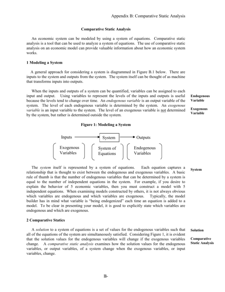
Appendix B: Comparative Static Analysis
Comparative Static Analysis
An economic system can be modeled by using a system of equations. Comparative static
analysis is a tool that can be used to analyze a system of equations. The use of comparative static
analysis on an economic model can provide valuable information about how an economic system
works.
1 Modeling a System
A general approach for considering a system is diagrammed in Figure B.1 below. There are
inputs to the system and outputs from the system. The system itself can be thought of as machine
that transforms inputs into outputs.
When the inputs and outputs of a system can be quantified, variables can be assigned to each
input and output. Using variables to represent the levels of the inputs and outputs is useful
because the levels tend to change over time. An endogenous variable is an output variable of the
system. The level of each endogenous variable is determined by the system. An exogenous
variable is an input variable to the system. The level of an exogenous variable is not determined
by the system, but rather is determined outside the system.
Endogenous
Variable
Exogenous
Variable
Figure 1: Modeling a System
Inputs
Exogenous
Variables
System
System of
Equations
Outputs
Endogenous
Variables
The system itself is represented by a system of equations.
Each equation captures a
relationship that is thought to exist between the endogenous and exogenous variables. A basic
rule of thumb is that the number of endogenous variables that can be determined by a system is
equal to the number of independent equations in the system. For example, if you desire to
explain the behavior of 5 economic variables, then you must construct a model with 5
independent equations. When examining models constructed by others, it is not always obvious
which variables are endogenous and which variables are exogenous. Typically, the model
builder has in mind what variable is “being endogenized” each time an equation is added to a
model. To be clear in presenting your model, it is good to explicitly state which variables are
endogenous and which are exogenous.
System
2 Comparative Statics
A solution to a system of equations is a set of values for the endogenous variables such that
all of the equations of the system are simultaneously satisfied. Considering Figure 1, it is evident
that the solution values for the endogenous variables will change if the exogenous variables
change. A comparative static analysis examines how the solution values for the endogenous
variables, or output variables, of a system change when the exogenous variables, or input
variables, change.
B1
Solution
Comparative
Static Analysis
Appendix B: Comparative Static Analysis
A major difficulty in analyzing a complicated system is identifying cause and effect. With many
endogenous and exogenous variables changing simultaneously, it is difficult to uncover how a
change in a single input variable affects the outputs of the system. For this reason, it is standard
practice when performing comparative static analyses to examine the changes in the solutions for
the endogenous variables that occur when one exogenous variable is increased by one unit.
Comparative
Static Multiplier
A comparative static multiplier gives the change in a chosen endogenous variable when a
chosen exogenous variable increases by one unit. Thus, if there are 5 endogenous variables and
7 exogenous variables in a model, then (5)(7) = 35 comparative static multipliers can be
calculated. In this book, the comparative static multiplier for an endogenous variable y given a
one unit increase in an exogenous variable x is written y/x, mathematically recognizing that the
multiplier is the partial derivative of the endogenous variable take with respect to the exogenous
variable.
When the system of equations being analyzed can be solved, the following five step approach
can used to perform a comparative static analysis:
1. Write down the model as a system of equations.
2. Classify the variables in model.
 Identify the endogenous variables in model. The number of endogenous variables
should be equal to the number of independent (or nonequivalent) equations in the
model.
 Classify the remaining variables as exogenous variables.
3. Solve the model: Find the solution for each endogenous variable as a function of the model's
exogenous variables.
4. Calculate the comparative static multipliers.
 Choose an endogenous variable of interest.
 Choose an exogenous variable of interest.
 Take the derivative of the solution for the endogenous variable with respect to the
exogenous variable of interest.
 Use different endogenous and exogenous variable combinations until all the desired
comparative static multipliers have been found.
5. Interpret each comparative static multiplier calculated as the change in the endogenous
variable of interest that occurs when the exogenous variable of interest increases by one unit.
Those who are not very familiar with calculus may find the mathematics of comparative static
analysis overwhelming. For those in this situation, the preferable course of action would be to
learn the mathematics since some results can only be obtained using the mathematics. (A good
first step would be to carefully study the mathematical appendix of this book.) However, many
comparative static results can be obtained using graphical tools. Thus, even those who cannot
calculate derivatives can do comparative static analyses.
The example in the next section will help make the general ideas discussed in this section and
the last section more concrete.
3 An Example: A Market for a Product
Suppose you want to develop a model of a market for a product. We do not have to specify the
product. We need only know that the market is for an output of a production process (i.e., a good
2
Appendix B: Comparative Static Analysis
or service) as opposed to an input (e.g., labor). A market always involves an interaction between
buyers and sellers. A model of a market for a specific product can be developed using a system
of equations as follows. First, develop an equation to describe the behavior of buyers. Second,
develop an equation to describe the behavior of sellers. Finally, develop an equation to describe
the interaction of buyers and sellers.
Although many factors may affect the willingness of buyers to buy a product, let's only
consider two here: price and income. Let the variable D denote the demand for the product (i.e.,
the amount of the product which buyers wish to buy); let P denote the price of the product; and
let Y denote the income of buyers. Typically, an increase in price leads to a decrease in demand,
while an increase in income leads to an increase in demand. These assumptions are captured by
the following linear equation:
D  aY  bP , a  0 , b  0 .
The variables a and b are called sensitivity parameters. The variable a measures the
sensitivity of demand to a change in income, while the variable b measures the sensitivity of
demand to a change in price. To understand why these variables measure sensitivity, substitute
in numbers for the variables Y, P, a, and b. Let Y = 100, P = 3, a = .5, and b = 2. Given these
numbers, D = (.5)(100) - (2)(3) = 44. Now, note that if Y increases by 1 (from 100 to 101) then
D increases by a = .5 (from 44 to 44.5), while if P increases by 1 (from 3 to 4) then D decreases
by b = 2 (from 44 to 42). This example illustrates that the parameter a gives the change in
demand that occurs when income increases by one unit, while the parameter b gives the change
in demand that occurs when the product price increases by one unit. If the sensitivity parameter
a were equal to zero, then demand would be totally insensitive to a change in income. If the
sensitivity parameter b were equal to zero, then demand would be totally insensitive to a change
in price. As the sensitivity parameter a gets larger, demand becomes more responsive to a
change in income. As the sensitivity parameter b gets larger, demand becomes more responsive
to a change in price.
The demand curve is graphed in Figure 2, with P being treated as the independent variable
and D being treated as the dependent variable. The demand curve is linear. The intercept of the
demand curve is equal to aY and is found by setting independent variable P equal to zero. The
slope of the demand curve is -b, equal to the coefficient on the independent variable P.
Figure 2: The Demand Curve
D
aY
Slope  b
D  aY  bP
P
B3
Sensitivity
Parameter
Appendix B: Comparative Static Analysis
Considering the willingness of sellers to produce and sell a product, assume that only the
product price is important. Let the variable S denote the supply of the product (i.e., the amount
of the product which sellers wish to sell), and let P denote the price of the product as before.
Typically, an increase in price leads to an increase in supply. This assumption is captured by the
equation:
S  cP , c  0 .
The supply curve is graphed in Figure 3, with P being treated as the independent variable and
S being treated as the dependent variable. The supply curve is linear. The intercept of the
supply curve is equal to zero, found by setting independent variable P equal to zero. The slope of
the supply curve is c, equal to the coefficient on the independent variable P. The variable c is a
sensitivity parameter, giving the change in supply that occurs when the price increases by one
unit.
Figure 3: The Supply Curve
S
S  cP
Slope  c
P
Equilibrium
Condition
The market is represented in Figure B.4, where the supply and demand curves are each plotted
in the same space. The supply and demand curves are each plotted with the price variable P as
the independent variable. Examining the figure, note that supply exceeds demand when the price
is above the price P*, meaning there is a surplus of the product. Alternatively, demand exceeds
supply when the price is below the price P*, meaning there is a shortage of the product. If there
was a surplus, we might expect the price to decrease. Alternatively, if there was a shortage, we
might expect the price to increase. Consequently, we would expect the price to gravitate toward
the price P* where supply equals demand. This notion can be captured by our model by adding
the equilibrium condition S = D.
4
Appendix B: Comparative Static Analysis
Figure 4: The Market
S, D
S  cP
aY
S *  D*
D  aY  bP
P*
P
Examining Figure 4, notice that the equilibrium condition, together with demand equation and
supply equation, determines the price P. That is, there is only one price such that supply equals
demand---the equilibrium price P*. Thus, P is an endogenous variable. As shown on the vertical
axis in Figure 2.4, the equilibrium quantity supplied S* and the equilibrium quantity demanded D*
are also determined by the three equations of the model. Thus, the variables S and D are also
endogenous variables.
To summarize, the model consists of the three equations that determine the three endogenous
variables S, D, and P. The remaining variables Y, a, b, and c are exogenous. The following
presentation of the model is useful in that it is brief and complete once the definitions of the
variables are understood:
(B.1) D  aY  bP , a  0 , b  0 ;
(B.2) S  cP , c  0 ;
(B.3) S  D .
Classification of Variables (7): P, S, D, Y, a, b, c
Endogenous Variables (3): P, S, D
Exogenous Variables (4): a, b, c, Y.
To solve the model, remember that the goal is to isolate each endogenous variable on one side
of an equation and have only exogenous variables on the other side. The abbreviations ST, AT,
and MT used in the solutions below stand for the substitution theorem, the addition theorem, and
the multiplication theorem. These theorems are explained in Appendix A---the mathematical
appendix. The mathematical appendix also contains an example of how to apply these theorems
to solve a system of equations. It is generally easiest to solve models representing markets by
starting with the equilibrium condition. In this case, by starting with the equilibrium condition,
the solution for P can be found:
SD
cP  aY  bP ,
bP  cP  aY ,
[b  c]P  aY ,
a
P
Y,
bc
Given (B.3)
ST, (B.1), (B.3)
AT
Distributive Law
MT
B5
Equilibrium
Price
Appendix B: Comparative Static Analysis
Notice that the solution for P was found by applying the substitution theorem first, the
addition theorem second, and the multiplication theorem last. Those who have had some practice
solving systems of equations know that it is quite possible to “go around in circles” and never
reach a solution. As a general rule, applying the theorems in the order used here is best in terms
of making progress toward a solution.
Having found the solution for P, the solutions for D can now be found by substitution as
follows:
D  aY  bP ,
a
D  aY  b
Y,
bc
bc
a
Da
Y b
Y,
bc
bc
ac
D
Y
bc
Given (1)
ST, Solution for P
Multiply aY term by
bc
 1.
bc
Combine terms
The solution for S can then be easily found:
S  D,
ac
S
Y
bc
Given (3)
ST, Solution for D
The solution for P is associated with P* on the horizontal axis of Figure B.4. It is the only
price that satisfies equations (B.1), (B.2), and (B.3) simultaneously. The solutions for S and D
are associated with S* and D* on the vertical axis of Figure B.4. Again, only these solutions are
consistent with equations (B.1), (B.2), and (B.3) holding simultaneously.
The solution is the model’s predicted value of the endogenous variable. Thus, this model can
predict the product price and the quantity of product bought and sold. Note, however, that each
solution depends upon the exogenous variables of the model. Values for the exogenous variables
must be given before the model can generate the predictions for the endogenous variables. If,
for example, it was known that a = .5, b = 3, c = 2, and Y = 100, then we can obtain our model's
predictions for the variables P, S, and D from the solutions above:
P
a
.5
Y
100  10
bc
3 2
and
SD
ac
(.5)( 2)
Y
100  20 .
bc
3 2
Thus, given these particular values for the parameters a, b, and c, 20 units would be bought and
sold at a price of 10 (dollars) per unit.
However, if the exogenous variables change, then the predicted values of the endogenous
variables will change. The comparative static multiplier P/Y shows the effect that the
6
Appendix B: Comparative Static Analysis
exogenous variable Y has on the endogenous variable P through the system.1 This multiplier can
be calculated as follows:
P   a 

Y ,
Y Y  b  c 
a 

Y  ,
b  c Y

ST, Solution for P
Constant Coefficient Rule
a
.
bc
Power Rule
The result P / Y  a / [b  c] indicates that a one unit increase in Y leads to an increase in P
of a/[b+c]. If a = .5, b = 3, and c = 2, the result would indicate that a one dollar increase in
income would lead to increase in the product's price of a/[b+c] = .5/[3+2] = .10, or 10 cents.
To show this comparative static result graphically, note that when Y increases the intercept of
the demand curve in Figure 4 increases. Thus, as is shown in Figure 5, an increase in Y makes
the demand curve shift upward. As Y increases from Y1 to Y2, the equilibrium price level
increases from P1 to P2. Notice in the figure that the equilibrium quantity bought and sold also
increases. The reader should be able to confirm this by showing that the comparative static
multipliers D / Y and S / Y are positive.
Figure 5: The Effect of an increase in Y
S, D
aY2
S  cP
aY1
S2  D2
S1  D1
D  aY2  bP
D  aY1  bP
P1 P2
P
The comparative static multiplier P / c shows the effect that the exogenous variable c has
on the endogenous variable P through the system. This multiplier can be calculated as follows:
P   a 

Y ,
c c  b  c 
  1 
 aY 
,
c  b  c 
ST, Solution for P
Constant Coefficient Rule
1
See the mathematical appendix---Appendix A---for an explanation of how to calculate comparative static
multipliers using the rules of differentiation.
B7
Appendix B: Comparative Static Analysis



1
b  c ,

c
2
 aY 1b  c ,
 aY

 0.
b  c2
 aY
Algebra
Power Rule
Algebra
The result P / c   aY / [b  c]2 indicates that a one unit increase in c leads to a decrease in
P of aY / [b  c]2 .
To show this comparative static result graphically, note that when c increases the slope of the
supply curve in figure 2.4 increases. Thus, as is shown in Figure 6, an increase in c makes the
supply curve rotate upward. As c increases from c1 to c2, the equilibrium price level decreases
from P1 to P2. Notice in the figure that the equilibrium quantity bought and sold increases. The
reader should be able to confirm this by showing that the comparative static multipliers
D / c and S / c are positive.
Figure 6: The Effect of an increase in c
S, D
S  c2 P
S  c1P
S2  D2
S1  D1
D  aY  bP
P1
P2
P
A total of 12 comparative static multipliers can be calculated. For practice, the reader might
calculate and interpret these results. In addition, the reader should be able to show each of the
comparative static results diagrammatically.
Key Words: Appendix B
Endogenous Variable
System
Comparative Static Analysis
Sensitivity Parameter
Equilibrium Price
Exogenous Variable
Solution
Comparative Static Multiplier
Equilibrium Condition
Key Concepts: Appendix B


Modeling an economic system using a system of equations.
Performing a comparative static analysis.
8
Appendix B: Comparative Static Analysis
Review Questions: Appendix B
1. The following equations can be used to represent a model of a “capital market.” Solve this
system of equations, assuming the endogenous variables are AD, C, I, AS, S, Y.
(1) AD  C  I
(2) C  C  cY , C  0 , 0  c  1
(3) I  I  bi , I  0 , i  0 , b  0
(4) AS  AE
(5) Y  C  S
(6) AE  AD
2. The following equations can be used to represent a model of a “money market.” Solve this
system of equations, assuming the endogenous variables are Md, Ms, and i.
(1) M d / P  kY  hi ,
(2) M  M ,
(3) M d  M s .
s
k  0,
M0
h  0,
Y  0;
3. For the capital market model presented in question 1, plot consumption C as it depends upon
output Y (equation 2), and graph investment I as it depends upon the real interest rate
level I (equation 3). Identify the intercept and slope for each curve you draw. Give an
economic interpretation of the intercept and slope for each curve you have drawn.
4. Find and give economic interpretations of the multipliers Y / C and C / c for the capital
market model presented in question 1.
5. Find and give economic interpretations of the multipliers i /  M and i / h for the money
market model presented in question 1.
6. Assuming C  0 , 0  c  1,   0 , i  0 , and T  0 , plot the following equations in a
single
(Y,C)
coordinate
C  C  cY  T   i .
plane:
C C,
B9
C  C  cY ,
C  C  cY  T  ,