Operations and Production Management
MGMT 405
Answer set 3
MGMT 405 Operations and Production Management
Answer set 3
(Reference chapter 3– William J. Stevenson-2007, ninth edition)
Problems and Solutions
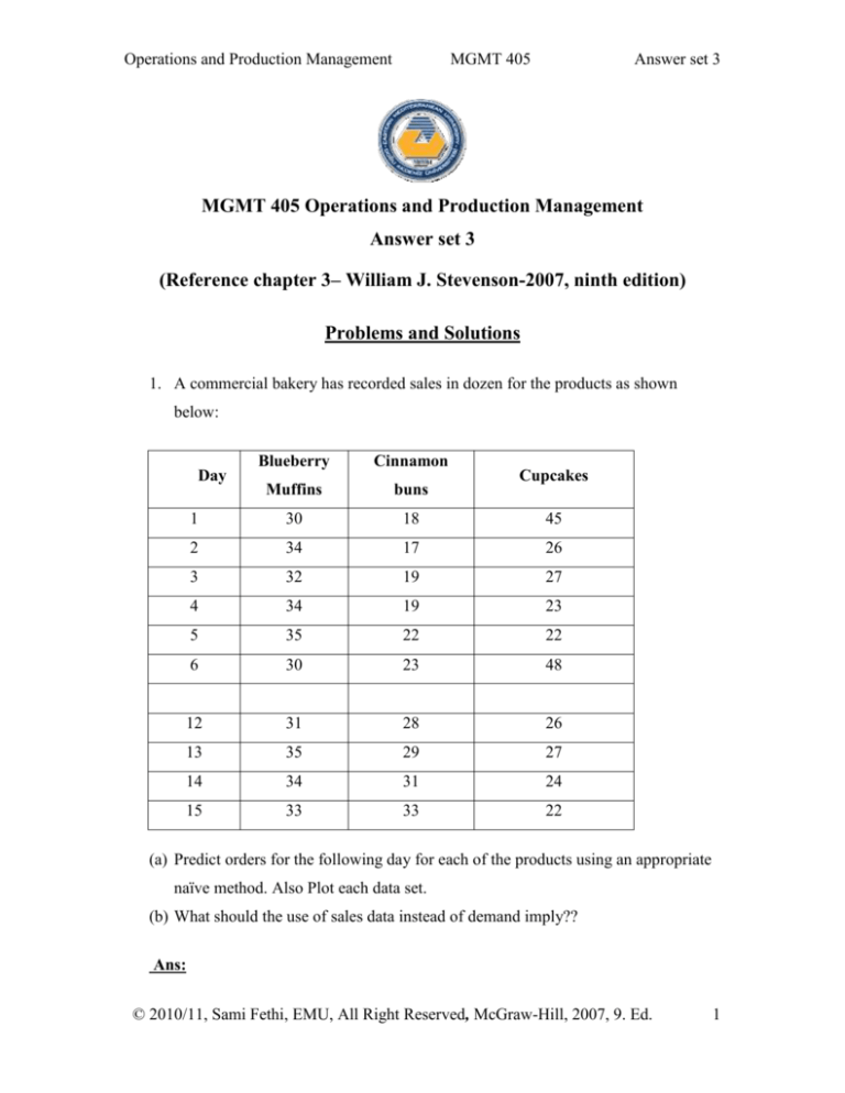
1. A commercial bakery has recorded sales in dozen for the products as shown
below:
Blueberry
Cinnamon
Muffins
buns
1
30
18
45
2
34
17
26
3
32
19
27
4
34
19
23
5
35
22
22
6
30
23
48
12
31
28
26
13
35
29
27
14
34
31
24
15
33
33
22
Day
Cupcakes
(a) Predict orders for the following day for each of the products using an appropriate
naïve method. Also Plot each data set.
(b) What should the use of sales data instead of demand imply??
Ans:
© 2010/11, Sami Fethi, EMU, All Right Reserved, McGraw-Hill, 2007, 9. Ed.
1
Operations and Production Management
MGMT 405
Answer set 3
(a) We need to use naive methods. This means that any simple appropriate method
can conducted. For example: Ploting each data set reveals that muffins orders are
almost stable, varying around an average (e.g. 33). The demand for cinnamon buns
has a trend. If we get the last three period, we realized that number increased two by
two so 33-31=2 and last one is 33+2=35. This is for the following day for cinnamon
buns. Demand for cupcakes has an apparent seasonal variation with peaks every five
days. Day 1=45, Day 6=48, Day 11=47 and the next peak would be Day 16=50.
A commercial bakery
60
sales
50
40
Blueberry Muffins
30
Cinnamon buns
20
Cupcakes
10
0
1
2
3
4
5
6
12
13
14
15
Days
(b) The use of sales data instead of demand implies that sales adequately reflect
demand. We are assuming that n stock-outs because demand equals sales if there are
no shortages.
2. A company records indicates that monthly sales for a seven-month period are
as follows:.
Month
Sales (000, unit)
Feb
19
Mar
18
Apr
15
© 2010/11, Sami Fethi, EMU, All Right Reserved, McGraw-Hill, 2007, 9. Ed.
2
Operations and Production Management
MGMT 405
May
20
Jun
18
July
22
Aug
20
Answer set 3
(a) Plot the monthly data as can be seen in the table above.
(b) Forecast the monthly sales using linear trend equation,
(c) A five-month moving average and exponential Smoothing technique? Assume
that smoothing constant and march forecast value are 0.20 and 19 respectively.
(d) The naïve approach
(e) A weight average method conducting 0.60 for August, 0.30 for July, and 0.10 for
June.
(f) Which method seems least appropriate? Why?
Ans:
(a)
Sales
25
000
20
15
Sales
10
5
0
Feb
Mar
Apr
May
Jun
July
Aug
month
© 2010/11, Sami Fethi, EMU, All Right Reserved, McGraw-Hill, 2007, 9. Ed.
3
Operations and Production Management
MGMT 405
Answer set 3
(b)
T (or x)
Square of t
Y
tY
1
1
19
19
2
4
18
36
3
9
15
45
4
16
20
80
5
25
18
90
6
36
22
132
7
49
20
140
Sum= 28
Sum of square= 140
Sum= 132
Sum= 542
n= 7
 x  y- x xy
n  x -(  x)
2
a=
2
b=
2
n xy-  x y
n  x 2 -(  x)2
Or
If formula b is used first, it may be used formula a in the following format:
n xy   x y
n x 2   x 
2
a
Y  b  X
n
b
7(542)  28(132)
 0.50
7(140)  28(28)
a
132  0.50(50)
 16.86
7
Y = 16.86 + 0.50X
After Aug (7), For sept: Y = 16.86 + 0.50(8)=20.86
(b) MA5 
15  18  22  20
 19
5
© 2010/11, Sami Fethi, EMU, All Right Reserved, McGraw-Hill, 2007, 9. Ed.
4
Operations and Production Management
MGMT 405
Answer set 3
(c) Ft = Ft-1 + (At-1 - Ft-1)
Ft = forecast for period t
Ft-1 = forecast for the previous period
= smoothing constant
At-1 = actual data for the previous period
April-F=19+0.20(18-19)=18.8
May- F=18.8+0.20(15-18.8)=18.04
June- F=18.04+0.20(20-18.04)=18.43
July- F=18.43+0.20(18-18.43)=18.34
Aug- F=18.34+0.20(22-18.34) =19.07
Sep- F=19.07+0.20(20-19.07) =19.26
(d) It may be around 20 (19.26)
(e) WA=0.60 (20) + 0.30 (22) + 0.10 (18) =20.4
(f) Probably trend method because the data appear to vary around Y = 16.86 +
0.50(4) =18.86.
3. A cosmetics manufacturer’s marketing department has developed a linear trend
equation that can be used to predict annual sales of its popular hand-foot cream.
Ft = 80 + 15 t
Where Ft =Annual sales (000 bottles), and assume that t= 0 in1990
(a) Are annual sales increasing or decreasing? By how much.
© 2010/11, Sami Fethi, EMU, All Right Reserved, McGraw-Hill, 2007, 9. Ed.
5
Operations and Production Management
MGMT 405
Answer set 3
(b) Predict annual sales for the year 2006 using the equation.
(c ) Predict changes in annual sales the year between 1995 and 2005 using the
equation.
Ans:
(a) Ft = 80 + 15 t
15 is the slope of the equation so this value show us whether annual sales increase or
decrease. The sign of the value is positive that’s why annual sales are increasing by
15000 bottles per year.
(b) Ft = 80 + 15 t= 80+ 15(16) = 320000
Where t=2006-1990=16
(c) Ft = 80 + 15 t= 80+ 15(5) = 155000 in 1995
Ft = 80 + 15 t= 80+ 15(15) = 305000 in 2005
Change in sales between the relevant years= 305000-155000=150000
4. New Car sales with monthly indexes (seasonal relatives) for a dealer for the past
years are shown in the following table:
Month
Unit sold
index
Month
Unit sold
index
Jan
640
0.8
Jul
765
0.9
Feb.
648
0.8
Aug
805
1.15
Mar
630
0.7
Sept
840
1.20
© 2010/11, Sami Fethi, EMU, All Right Reserved, McGraw-Hill, 2007, 9. Ed.
6
Operations and Production Management
MGMT 405
Answer set 3
Apr
761
0.94
Oct
828
1.20
May
735
0.89
Nov
840
1.25
Jun
850
1.00
Dec
800
1.25
(a) Plot the data. Does there seem to be a trend?
sales volume
Unit Sales
900
800
700
600
500
400
300
200
100
0
Unit sold
index
Jan Feb. Mar Apr May Jun
Jul
Aug Sept Oct Nov Dec
Month
It seems that there exists a trend starting from 600 to 800.
(b) Compute the Deseasonalized car sales
Month
Unit sold
index
Deseasonalize =actual sales/seasonal relative
Jan
640
0.8
640/0.8=800
Feb.
648
0.8
810
Mar
630
0.7
900
Apr
761
0.94
809.6
May
735
0.89
825.8
© 2010/11, Sami Fethi, EMU, All Right Reserved, McGraw-Hill, 2007, 9. Ed.
7
Operations and Production Management
MGMT 405
Jun
850
1.00
850
Jul
765
0.9
850
Aug
805
1.15
700
Sept
840
1.20
700
Oct
828
1.20
690
Nov
840
1.25
672
Dec
800
1.25
640
Answer set 3
(c ) Plot both seasonalized and Deseasonalized car sales data on the same graph. Briefly
explain.
sales
1000
volume
800
seasonal
600
index
400
deseasonal
200
0
Jan Feb. Mar
Apr May Jun
Jul
Aug Sept Oct
Nov Dec
Month
Seasonalized car sales data are upward trend in sales and Deseasonalized car sales data
are downward trend in sales.
5. Two different forecast techniques (F1 and F2) were used to forecast demand for
cases of bottled water. Actual demand the two sets of forecasts are as follows:
Period and Demand
Predicted Demand
Period
Unit sold
F1
F2
1
68
66
66
© 2010/11, Sami Fethi, EMU, All Right Reserved, McGraw-Hill, 2007, 9. Ed.
8
Operations and Production Management
MGMT 405
2
75
68
68
3
70
72
70
4
74
71
72
5
69
72
74
6
72
70
76
7
80
71
78
8
78
74
80
Answer set 3
(a) Compute MAD for each set of forecast. Which forecast is better or appears to be
more accurate? Briefly explain.
(b) Compute MES for each set of forecast. Which forecast is better or appears to be
more accurate? Briefly explain.
(c) Compute MAPE for each set of forecast. Which forecast is better or appears to be
more accurate? Briefly explain.
(d) Compute a tracking signal for the 8th month for each forecast using the
cumulative error for 1 and 8.
(e) Compute 2s control limits for each forecast.
Ans:
Period
Demand
F1
e
e
e2
( e /actual)*100
1
68
66
2
2
4
3
2
75
68
7
7
49
9.3
3
70
72
-2
2
4
2.8
4
74
71
3
3
9
4
5
69
72
-3
3
9
4.3
6
72
70
2
2
4
2.7
7
80
71
9
9
81
11.2
8
78
74
4
4
16
5.1
32
176
42.4
586
© 2010/11, Sami Fethi, EMU, All Right Reserved, McGraw-Hill, 2007, 9. Ed.
9
Operations and Production Management
Period
Demand
F2
MGMT 405
e
e
Answer set 3
e2
( e /actual)*10
0
1
68
66
2
2
4
3
2
75
68
7
7
49
10.2
3
70
70
0
0
0
0
4
74
72
2
2
4
2.7
5
69
74
-5
5
25
6.7
6
72
76
-4
4
16
5.2
7
80
78
2
2
4
2.5
8
78
80
-2
2
4
2.5
24
106
32.9
(a) Compute MAD for each set of forecast. Which forecast is better or appears to be
more accurate? Briefly explain.
Ans:
MAD= ∑│Actual-Forecast│/n
MADF1= 32/8= 4
© 2010/11, Sami Fethi, EMU, All Right Reserved, McGraw-Hill, 2007, 9. Ed.
10
Operations and Production Management
MGMT 405
Answer set 3
MADF2= 24/8= 3
F2 forecast results appears to be more accurate because MAD model gives less error
than F1.
(b) Compute MES for each set of forecast. Which forecast is better or appears to be
more accurate? Briefly explain.
Ans:
MES= ∑│Actual-Forecast│2/ (n-1)
MESF1= 176/7= 25.14
MESF2= 106/7= 15.14
F2 forecast results appears to be more accurate because MES model gives less error
than F1.
(c) Compute MAPE for each set of forecast. Which forecast is better or appears to be
more accurate? Briefly explain.
Ans:
MAPE= (∑ (│Actual-Forecast│/actual)*100)/n
MAPE F1=42.4/8=5.34
MAPE F2==32.9/8=4.11
F2 forecast results appears to be more accurate because MAPE model gives less error
than F1.
(d) Compute a tracking signal for the 8th month for each forecast using the cumulative
error as well as limits of ± 4 for 1 and 8.
© 2010/11, Sami Fethi, EMU, All Right Reserved, McGraw-Hill, 2007, 9. Ed.
11
Operations and Production Management
MGMT 405
Answer set 3
Ans:
Tracking Signalt = ∑ (Actual-Forecast)/MADt
MSE
Control Limits= 0 +/- 2
CUM
Period
Demand
F1
e
e
1
68
66
2
2
2
2
75
68
7
7
9
3
70
72
-2
2
7
4
74
71
3
3
10
5
69
72
-3
3
7
6
72
70
2
2
9
7
80
71
9
9
18
8
78
74
4
4
22
ERROR
CUM
Period
Demand
F2
e
e
1
68
66
2
2
2
2
75
68
7
7
9
3
70
70
0
0
9
4
74
72
2
2
11
5
69
74
-5
5
6
6
72
76
-4
4
2
7
80
78
2
2
4
8
78
80
-2
2
2
ERROR
MADF1= 32/8= 4
© 2010/11, Sami Fethi, EMU, All Right Reserved, McGraw-Hill, 2007, 9. Ed.
12
Operations and Production Management
MGMT 405
Answer set 3
MADF2= 24/8= 3
MESF1= 176/7= 25.14
MESF2= 106/7= 15.14
MAPE F1=42.4/8=5.34
MAPE F2==32.9/8=4.11
Tracking Signalt = ∑ (Actual-Forecast)/MADt =cumulative error/ MADt
Tracking Signalt for F1= 22/4=5.5
Tracking Signalt for F2= 2/3=0.66
Tracking Signal is used to monitor a forecast whether the method is biased or not.
Values can be positive or negative and zero value would be ideal. Since 5.5 >4 the
forecast method 1 is biased. This means that using F1, we are underestimating
(positive bias)* demand. Since 0.66 < 4, the forecast is in control.
*overestimating
(negative bias).
(e) Compute 2s control limits for each forecast.
Ans:
Control Limits= 0 +/- 2
MSE
Control Limits for F1 = 0 +/- 2
MSE =0 +/- 2 √(25.14=+10.01 and -10.01
Control Limits for F2 = 0 +/- 2
MSE =0 +/- 2 √(15.14=+7.78 and -7.78
Since all errors for both forecasts 1 and 2 are within these limits, the forecasts are in
control (see column e for both F1 and F2 in the tables above).
© 2010/11, Sami Fethi, EMU, All Right Reserved, McGraw-Hill, 2007, 9. Ed.
13