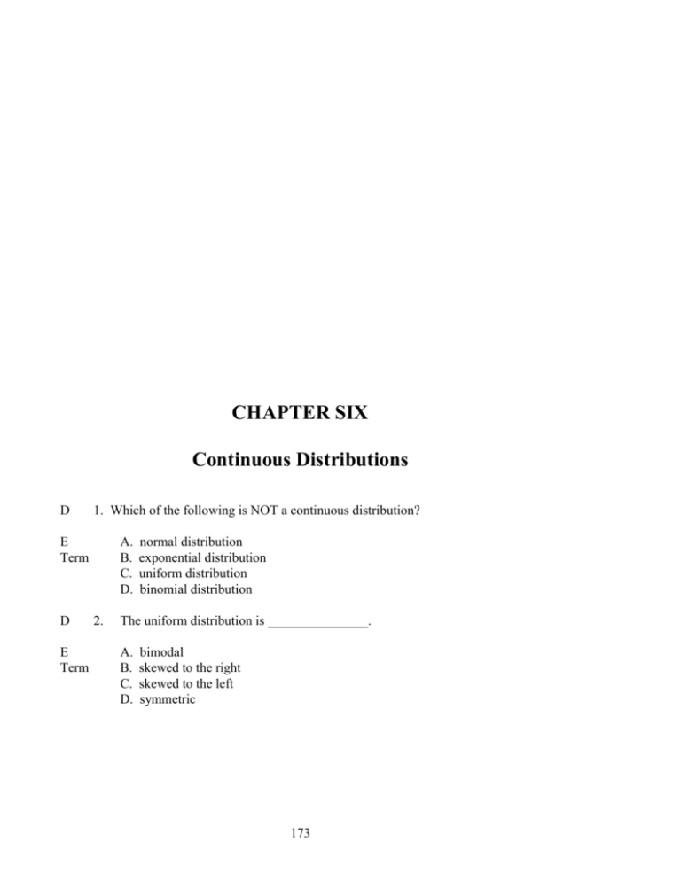
CHAPTER SIX
Continuous Distributions
D
1. Which of the following is NOT a continuous distribution?
E
Term
D
E
Term
A.
B.
C.
D.
2.
normal distribution
exponential distribution
uniform distribution
binomial distribution
The uniform distribution is _______________.
A.
B.
C.
D.
bimodal
skewed to the right
skewed to the left
symmetric
173
174
Test Bank
A
3.
E
Term
A.
B.
C.
D.
4.
rectangular distribution
gamma distribution
beta distribution
Erlang distribution
The distribution in the following graph is a ________ distribution.
f(X)
D
The uniform distribution is also known as the __________.
0.06
0.05
0.04
0.03
0.02
0.01
0.00
35
E
Term
A
E
Term
A.
B.
C.
D.
5.
40
45
50
55
60 x 65
normal
gamma
exponential
uniform
The distribution in the following graph is a ________ distribution.
A.
B.
C.
D.
normal
gamma
exponential
uniform
Chapter 6: Continuous Distributions 175
C
6.
E
Term
B
A.
B.
C.
D.
7.
E
Term
A
8.
M
Calc
1/8
1/4
1/12
1/20
If X is uniformly distributed over the interval 8 to 12, inclusively (8  X  12),
then the mean() of this distribution is __________________.
A.
B.
C.
D.
9.
normal
gamma
exponential
uniform
If X is uniformly distributed over the interval 8 to 12, inclusively (8  X  12),
then the height of this distribution, f(x), is __________________.
A.
B.
C.
D.
M
Calc
C
The distribution in the following graph is a ________ distribution.
10
20
5
incalculable
If X is uniformly distributed over the interval 8 to 12, inclusively (8  X  12),
then the standard deviation () of this distribution is __________________.
A.
B.
C.
D.
4
1.33
1.15
2
176
Test Bank
B
10.
M
Calc
C
A.
B.
C.
D.
11.
M
Calc
D
12.
M
Calc
A
M
Calc
0.250
0.500
0.375
0.000
If X is uniformly distributed over the interval 8 to 12, inclusively (8  X  12),
then P(X < 7) is __________________.
A.
B.
C.
D.
14.
0.250
0.333
0.375
0.000
If X is uniformly distributed over the interval 8 to 12, inclusively (8  X  12),
then the P(13  X  15) is __________________.
A.
B.
C.
D.
13.
0.250
0.500
0.333
1.000
If X is uniformly distributed over the interval 8 to 12, inclusively (8  X  12),
then the P(10.0  X  11.5) is __________________.
A.
B.
C.
D.
M
Calc
B
If X is uniformly distributed over the interval 8 to 12, inclusively (8  X  12),
then the P(9  X  11) is __________________.
0.500
0.000
0.375
0.250
If X is uniformly distributed over the interval 8 to 12, inclusively (8  X  12),
then P(X  11) is __________________.
A.
B.
C.
D.
0.750
0.000
0.333
0.500
Chapter 6: Continuous Distributions 177
D
15.
E
Calc
A
A.
B.
C.
D.
16.
E
Calc
B
17.
M
Calc
C
M
Calc
50
25
10
5
If X is uniformly distributed over the interval 20 to 30, inclusively (20  X  30),
then the standard deviation () of this distribution is __________________.
A.
B.
C.
D.
19.
1/10
1/20
1/30
1/50
If X is uniformly distributed over the interval 20 to 30, inclusively (20  X  30),
then the mean () of this distribution is __________________.
A.
B.
C.
D.
18.
0.750
0.000
0.333
0.500
If X is uniformly distributed over the interval 20 to 30, inclusively (20  X  30),
then the height of this distribution, f(x), is __________________.
A.
B.
C.
D.
M
Calc
D
If X is uniformly distributed over the interval 8 to 12, inclusively (8  X  12),
then P(X  10) is __________________.
incalculable
8.33
0.833
2.89
If X is uniformly distributed over the interval 20 to 30, inclusively (20  X  30),
then P(25  X  28) is __________________.
A.
B.
C.
D.
0.250
0.500
0.300
1.000
178
Test Bank
A
20.
M
Calc
B
A.
B.
C.
D.
21.
M
Calc
C
22.
M
Calc
D
M
Calc
0.500
0.300
0.000
0.250
If X is uniformly distributed over the interval 20 to 30, inclusively (20  X  30),
then P(X  22) is __________________.
A.
B.
C.
D.
24.
0.500
0.000
0.375
0.200
If X is uniformly distributed over the interval 20 to 30, inclusively (20  X  30),
then P(X < 17) is __________________.
A.
B.
C.
D.
23.
0.250
0.333
0.375
0.000
If X is uniformly distributed over the interval 20 to 30, inclusively (20  X  30),
then P(33  X  35) is __________________.
A.
B.
C.
D.
M
Calc
A
If X is uniformly distributed over the interval 20 to 30, inclusively (20  X  30),
then P(21.75  X  24.25) is __________________.
0.200
0.300
0.000
0.250
If X is uniformly distributed over the interval 20 to 30, inclusively (20  X  30),
then P(X  24) is __________________.
A.
B.
C.
D.
0.100
0.000
0.333
0.600
Chapter 6: Continuous Distributions 179
C
25.
Helen Casner, a labor relations arbitrator, feels that the amount of time needed to
arbitrate a labor dispute is uniformly distributed over the interval 4 to 24 hours,
inclusively (4  X  24). Accordingly, the mean (average) time needed to
arbitrate a labor dispute is ____________.
M
BCalc
A.
B.
C.
D.
D
Helen Casner, a labor relations arbitrator, feels that the amount of time needed to
arbitrate a labor dispute is uniformly distributed over the interval 4 to 24 hours,
inclusively (4  X  24). Accordingly, the probability that a labor dispute will be
arbitrated in 8 hours or less is ____________.
26.
20 hours
16 hours
14 hours
12 hours
M
BCalc
A.
B.
C.
D.
C
Helen Casner, a labor relations arbitrator, feels that the amount of time needed to
arbitrate a labor dispute is uniformly distributed over the interval 4 to 24 hours,
inclusively (4  X  24). Accordingly, the probability that a labor dispute will
require between 8 and 16 hours, inclusively, for arbitration is ____________.
27.
0.3333
0.6667
0.0000
0.2000
M
BCalc
A.
B.
C.
D.
B
The normal distribution is an example of _______.
28.
E
Term
A.
B.
C.
D.
0.3333
0.6667
0.4000
0.2000
a discrete distribution
a continuous distribution
a bimodal distribution
an exponential distribution
180
Test Bank
B
29.
The total area underneath any normal curve is _______.
E
Term
A.
B.
C.
D.
D
The area to the left of the mean in any normal distribution is _______.
30.
equal to the mean
equal to 1
equal to the variance
equal to the coefficient of variation
E
Term
A.
B.
C.
D.
B
For any normal distribution, any value less than the mean would have a _______.
31.
equal to the mean
equal to 1
equal to the variance
equal to 0.5
E
Term
A.
B.
C.
D.
D
A standardized normal distribution has the following characteristics:
32.
positive Z-score
negative Z-score
negative variance
negative probability of occurring
E
Term
A.
B.
C.
D.
C
If X is a normal random variable with mean 80 and standard deviation 5, calculate
the Z score if X=88.
33.
E
Calc
D
E
Calc
A.
B.
C.
D.
34.
the mean and variance are both equal to 1
the mean and variance are both equal to 0
the mean is equal to the variance
the mean is equal to 0 and the variance is equal to 1
1.8
-1.8
1.6
-1.6
If X is a normal random variable with mean 80 and standard deviation 5, calculate
the Z score if X=72.
A.
B.
C.
D.
1.8
-1.8
1.6
-1.6
Chapter 6: Continuous Distributions 181
D
35.
E
Calc
C
A.
B.
C.
D.
36.
E
Calc
C
37.
M
Calc
B
E
Calc
63.4
56.6
66.8
53.2
Suppose X is a normal random variable with mean 60 and standard deviation 2.
A Z score was calculated for a number, and the Z score is -1.3. What is X?
A.
B.
C.
D.
39.
1.5
2.5
-1.5
-2.5
Suppose X is a normal random variable with mean 60 and standard deviation 2.
A Z score was calculated for a number, and the Z score is 3.4. What is X?
A.
B.
C.
D.
38.
2.1
12
1.2
2.4
If X is a normal random variable with mean 60 and standard deviation 2, calculate
the Z score if X=57.
A.
B.
C.
D.
M
Calc
D
If X is a normal random variable with mean 80 and standard deviation 5, calculate
the Z score if X=92.
58.7
61.3
62.6
57.4
Let Z be a normal random variable with mean 0 and standard deviation 1. Use the
normal tables to find P(Z < 1.3).
A.
B.
C.
D.
0.4032
0.9032
0.0968
0.3485
182
Test Bank
D
40.
E
Calc
C
A.
B.
C.
D.
41.
M
Calc
D
42.
M
Calc
C
M
Calc
0.4821
-0.4821
0.9821
0.0179
Let Z be a normal random variable with mean 0 and standard deviation 1. Use the
normal tables to find P(Z > -1.1).
A.
B.
C.
D.
44.
0.4918
0.9918
0.0082
0.4793
Let Z be a normal random variable with mean 0 and standard deviation 1. Use the
normal tables to find P(Z < -2.1).
A.
B.
C.
D.
43.
0.4032
0.9032
0.4893
0.0861
Let Z be a normal random variable with mean 0 and standard deviation 1. Use the
normal tables to find P(Z > 2.4).
A.
B.
C.
D.
M
Calc
B
Let Z be a normal random variable with mean 0 and standard deviation 1. Use the
normal tables to find P(1.3 < Z < 2.3).
0.3643
0.8643
0.1357
-0.1357
Let Z be a normal random variable with mean 0 and standard deviation 1. Use the
normal tables to find P(-2.25 < Z < -1.1).
A.
B.
C.
D.
0.3643
0.8643
0.1235
0.4878
Chapter 6: Continuous Distributions 183
B
45.
M
Calc
C
A.
B.
C.
D.
46.
E
Calc
A
47.
M
Calc
A
M
Calc
0.670
-1.254
0.000
1.280
Let Z be a normal random variable with mean 0 and standard deviation 1. The 90th
percentile of Z is ____________.
A.
B.
C.
D.
49.
0.670
-1.254
0.000
1.280
Let Z be a normal random variable with mean 0 and standard deviation 1. The 75th
percentile of Z is ____________.
A.
B.
C.
D.
48.
0.3643
0.8521
0.1235
0.4878
Let Z be a normal random variable with mean 0 and standard deviation 1. The 50th
percentile of Z is ____________.
A.
B.
C.
D.
M
Calc
D
Let Z be a normal random variable with mean 0 and standard deviation 1. Use the
normal tables to find P(-2.25 < Z < 1.1).
1.645
-1.254
1.960
1.280
Let Z be a normal random variable with mean 0 and standard deviation 1. The 95th
percentile of Z is ____________.
A.
B.
C.
D.
1.645
-1.254
1.960
1.280
184
Test Bank
B
50.
M
Calc
C
A.
B.
C.
D.
51.
M
Calc
B
52.
M
Calc
B
E
Calc
0.0987
0.4013
-0.0987
0.5987
Let X be a normal random variable with mean 20 and standard deviation 4. Find
P(16 < X < 22).
A.
B.
C.
D.
54.
0.2734
0.7734
0.2266
-0.2734
Let X be a normal random variable with mean 20 and standard deviation 4. Find
P(X < 19).
A.
B.
C.
D.
53.
0.3944
0.8944
0.1056
0.6056
Let X be a normal random variable with mean 20 and standard deviation 4. Find
P(X < 17).
A.
B.
C.
D.
M
Calc
D
Let X be a normal random variable with mean 20 and standard deviation 4. Find
P(X < 25).
0.4672
0.0328
0.1498
0.5328
Let X be a normal random variable with mean 20 and standard deviation 4. The
50th percentile of X is ____________.
A.
B.
C.
D.
4.000
20.000
22.698
26.579
Chapter 6: Continuous Distributions 185
C
55.
M
Calc
A
A.
B.
C.
D.
56.
M
Calc
D
57.
M
Calc
A
M
Calc
25.126
20.000
22.698
26.579
Let X be a normal random variable with mean 40 and standard deviation 8. Find
P(32 < X < 44).
A.
B.
C.
D.
59.
25.126
20.000
22.698
26.579
Let X be a normal random variable with mean 20 and standard deviation 4. The
95th percentile of X is ____________.
A.
B.
C.
D.
58.
25.126
20.000
22.698
26.579
Let X be a normal random variable with mean 20 and standard deviation 4. The
90th percentile of X is ____________.
A.
B.
C.
D.
M
Calc
D
Let X be a normal random variable with mean 20 and standard deviation 4. The
75th percentile of X is ____________.
0.4672
0.0328
0.1498
0.5328
Let X be a normal random variable with mean 40 and standard deviation 8. Find
P(X < 96).
A.
B.
C.
D.
1.0000
0.0000
0.0793
0.0575
186
Test Bank
B
60.
M
Calc
B
Let X be a normal random variable with mean 40 and standard deviation 2. Find
P(X < 28).
A.
B.
C.
D.
61.
1.0000
0.0000
0.2580
0.0472
A Z score is the number of __________ that a value is from the mean.
E
Term
A.
B.
C.
D.
C
Within a range of Z scores from -1 to +1, you can expect to find _______ per cent
of the values in a normal distribution.
62.
variances
standard deviations
units
miles
E
Term
A.
B.
C.
D.
A
Within a range of Z scores from -2 to +2, you can expect to find _______ per cent
of the values in a normal distribution.
63.
95
99
68
34
E
Term
A.
B.
C.
D.
C
The expected (mean) life of a particular type of light bulb is 1,000 hours with a
standard deviation of 50 hours. The life of this bulb is normally distributed.
What is the probability that a randomly selected bulb would last longer than 1150
hours?
M
Calc
64.
A.
B.
C.
D.
95
99
68
34
0.4987
0.9987
0.0013
0.5013
Chapter 6: Continuous Distributions 187
B
65.
M
Calc
C
A.
B.
C.
D.
66.
M
Calc
D
67.
H
Calc
0.3849
0.8849
0.1151
0.6151
Suppose you are working with a data set that is normally distributed with a mean
of 400 and a standard deviation of 20. Determine the value of X such that 60% of
the values are greater than X.
A.
B.
C.
D.
68.
0.4772
0.9772
0.0228
0.5228
The expected (mean) life of a particular type of light bulb is 1,000 hours with a
standard deviation of 50 hours. The life of this bulb is normally distributed.
What is the probability that a randomly selected bulb would last fewer than 940
hours?
A.
B.
C.
D.
H
Calc
A
The expected (mean) life of a particular type of light bulb is 1,000 hours with a
standard deviation of 50 hours. The life of this bulb is normally distributed.
What is the probability that a randomly selected bulb would last fewer than 1100
hours?
404.5
395.5
405.0
395.0
Suppose you are working with a data set that is normally distributed with a mean
of 400 and a standard deviation of 20. Determine the value of X such that only
1% of the values are greater than X.
A.
B.
C.
D.
446.6
353.4
400.039
405
188
Test Bank
C
69.
H
Calc
C
A.
B.
C.
D.
70.
M
Calc
B
71.
H
Calc
0.3944
0.8944
0.1056
0.6056
The E.P.A. has reported that the average fuel cost for a particular type of
automobile is $800 with a standard deviation of $80. Fuel cost is assumed to be
normally distributed. If one of these cars is randomly selected, what is the
probability that the fuel cost for this car exceeds $760?
A.
B.
C.
D.
72.
432.9
396
367.1
404
The E.P.A. has reported that the average fuel cost for a particular type of
automobile is $800 with a standard deviation of $80. Fuel cost is assumed to be
normally distributed. If one of these cars is randomly selected, what is the
probability that the fuel cost for this car exceeds $900?
A.
B.
C.
D.
M
Calc
B
Suppose you are working with a data set that is normally distributed with a mean
of 400 and a standard deviation of 20. Determine the value of X such that 5% of
the values are less than X.
0.1915
0.6915
0.3085
0.8085
The E.P.A. has reported that the average fuel cost for a particular type of
automobile is $800 with a standard deviation of $80. Fuel cost is assumed to be
normally distributed. We would expect that only 10% of these cars would have an
annual fuel cost greater than _______.
A.
B.
C.
D.
820.0
902.4
808.0
812.8
Chapter 6: Continuous Distributions 189
A
73.
M
Calc
C
The E.P.A. has reported that the average fuel cost for a particular type of
automobile is $800 with a standard deviation of $80. Fuel cost is assumed to be
normally distributed. If a car is randomly selected, what is the probability that
fuel cost would be between $700 and $900?
A.
B.
C.
D.
74.
0.7888
0.8944
0.3944
0.1056
The net profit of an investment is normally distributed with a mean of $10,000
and a standard deviation of $5,000. The probability that the investor will not have
a net loss is _____________.
M
BCalc
A.
B.
C.
D.
B
The net profit of an investment is normally distributed with a mean of $10,000
and a standard deviation of $5,000. The probability that the investor will have a
net loss is _____________.
75.
0.4772
0.0228
0.9772
0.9544
M
BCalc
A.
B.
C.
D.
A
The net profit of an investment is normally distributed with a mean of $10,000
and a standard deviation of $5,000. The probability that the investor’s net profit
will be between $12,000 and $15,000 is _____________.
76.
M
BCalc
A.
B.
C.
D.
0.4772
0.0228
0.9772
0.9544
0.1859
0.3413
0.8413
0.4967
190
Test Bank
C
77.
The net profit of an investment is normally distributed with a mean of $10,000
and a standard deviation of $5,000. The probability that the investor’s net gain
will be at least $5,000 is _____________.
M
BCalc
A.
B.
C.
D.
A
Completion time (from start to finish) of a building remodeling project is
normally distributed with a mean of 200 work-days and a standard deviation of 10
work-days. The probability that the project will be completed within 185 workdays is ______.
78.
0.1859
0.3413
0.8413
0.4967
M
BCalc
A.
B.
C.
D.
D
Completion time (from start to finish) of a building remodeling project is
normally distributed with a mean of 200 work-days and a standard deviation of 10
work-days. The probability that the project will be completed within 215 workdays is _____.
79.
0.0668
0.4332
0.5000
0.9332
M
BCalc
A.
B.
C.
D.
A
Completion time (from start to finish) of a building remodeling project is
normally distributed with a mean of 200 work-days and a standard deviation of 10
work-days. The probability that the project will not be completed within 215
work-days is _____.
80.
M
BCalc
A.
B.
C.
D.
0.0668
0.4332
0.5000
0.9332
0.0668
0.4332
0.5000
0.9332
Chapter 6: Continuous Distributions 191
C
81.
Completion time (from start to finish) of a building remodeling project is
normally distributed with a mean of 200 work-days and a standard deviation of 10
work-days. The probability that the project will be completed within ____ workdays is 0.99.
M
BCalc
A.
B.
C.
D.
B
The length of steel rods produced by a shearing process are normally distributed
with  = 120 inches and  = 0.05 inch. Industry standards require the rods to be
between 119.90 and 120.15 inches, inclusively. The probability that a rod
produced by this process will conform to industry standards is ______________.
82.
211
187
223
200
M
BCalc
A.
B.
C.
D.
C
The length of steel rods produced by a shearing process are normally distributed
with  = 120 inches and  = 0.05 inch. Industry standards require the rods to be
between 119.90 and 120.15 inches, inclusively. Any rod longer than 120.15
inches is re-sheared. The probability that a rod produced by this process will
require re-shearing is ___________.
83.
0.9542
0.9759
0.9974
0.6826
M
BCalc
A.
B.
C.
D.
B
The length of steel rods produced by a shearing process are normally distributed
with  = 120 inches and  = 0.05 inch. Industry standards require the rods to be
between 119.90 and 120.15 inches, inclusively. Any rod shorter than 119.90
inches is scrapped (used in the next melt). The probability that a rod produced by
this process will be scrapped is ___________.
84.
M
BCalc
A.
B.
C.
D.
0.0458
0.0228
0.0013
0.0241
0.0458
0.0228
0.0013
0.0241
192
Test Bank
A
85.
The weights of aluminum castings produced by a process are normally distributed
with  = 2 pounds and  = 0.10 pound. Design specifications require the castings
to weigh between 1.836 and 2.164 pounds, inclusively. The probability that a
casting produced by this process will conform to design specifications is
_________.
M
BCalc
A.
B.
C.
D.
C
The weights of aluminum castings produced by a process are normally distributed
with  = 2 pounds and  = 0.10 pound. Design specifications require the castings
to weigh between 1.836 and 2.164 pounds, inclusively. Any casting weighing less
than 1.836 pounds is scrapped. The probability that a casting produced by this
process will be scrapped, due to under-weight, is _________.
86.
0.8990
0.4495
0.9974
0.9500
M
BCalc
A.
B.
C.
D.
C
The weights of aluminum castings produced by a process are normally distributed
with  = 2 pounds and  = 0.10 pound. Design specifications require the castings
to weigh between 1.836 and 2.164 pounds, inclusively. Any casting weighing
more than 2.164 pounds is re-worked. The probability that a casting produced by
this process will be re-worked, due to over-weight, is _________.
87.
0.1010
0.4495
0.0505
0.0010
M
BCalc
A.
B.
C.
D.
B
Let X be a binomial random variable with n=20 and p=.8. If we use the normal
distribution to approximate probabilities for this, we would use a mean of
_______.
E
Calc
88.
A.
B.
C.
D.
0.0010
0.1010
0.0101
0.0505
20
16
3.2
8
Chapter 6: Continuous Distributions 193
C
89.
M
Calc
B
Let X be a binomial random variable with n=20 and p=.8. If we use the normal
distribution to approximate probabilities for this, we would use a standard
deviation of _______.
A.
B.
C.
D.
90.
16
3.2
1.79
0.16
Let X be a binomial random variable with n=20 and p=.8. If we use the normal
distribution to approximate probabilities for this, a correction for continuity
should be made. To find the probability of more than 12 successes, we should
find _______.
M
Term
A.
B.
C.
D.
B
Let X be a binomial random variable with n=20 and p=.8. If we use the normal
distribution to approximate probabilities for this, a correction for continuity
should be made. To find the probability of 12 successes or more, we should find
_______.
91.
P(X>12)
P(X>12.5)
P(X>11.5)
P(X<11.5)
M
Term
A.
B.
C.
D.
C
Let X be a binomial random variable with n=20 and p=.8. If we use the normal
distribution to approximate probabilities for this, a correction for continuity
should be made. To find the probability of more than 6 but less than 12 successes,
we should find _______.
H
Calc
92.
A.
B.
C.
D.
P(X>12)
P(X>11.5)
P(X>12.5)
P(X<12.5)
P(6<X<12)
P(6.5<X<12.5)
P(6.5<X<11.5)
P(5.5<X<12.5)
194
Test Bank
C
93.
Ten percent of all personal loans granted by First Easy Money Bank are defaulted
in the fourth re-payment month. One-hundred four-month old personal loans are
randomly selected from a population of 3,000. The number of defaulted loans in
this sample has a binomial distribution. If we use the normal distribution to
approximate probabilities for this, we would use a mean of _______.
M
BCalc
A.
B.
C.
D.
B
According to the U. S. Department of Commerce, 8.6% of the total civilian
employment in Washington state is related to manufactured exports. A sample of
200 civilian employees in Washington state is randomly selected. If X is the
number of employees in the sample with jobs related to manufactured exports,
then the mean (expected) value of X is _______________.
94.
30
50
10
300
M
BCalc
A.
B.
C.
D.
D
According to the U. S. Department of Commerce, 8.6% of the total civilian
employment in Washington state is related to manufactured exports. A sample of
200 civilian employees in Washington state is randomly selected. If X is the
number of employees in the sample with jobs related to manufactured exports,
then the standard deviation of X is _______________.
95.
H
Calc
D
A.
B.
C.
D.
96.
H
BCalc
8.60
17.20
15.72
3.96
8.60
17.20
15.72
3.96
According to the U. S. Department of Commerce, 8.6% of the total civilian
employment in Washington state is related to manufactured exports. A sample of
200 civilian employees in Washington state is randomly selected. The probability
that between 9 and 15 (inclusively) of the employees have jobs related to
manufactured exports is _______________.
A.
B.
C.
D.
0.9564
0.9435
0.9386
0.9874
Chapter 6: Continuous Distributions 195
B
97.
The exponential distribution is an example of _______.
E
Term
A.
B.
C.
D.
B
If arrivals at a bank follow a Poisson distribution, then the time between arrivals
would be _______.
98.
M
Term
B
99.
a discrete distribution
a continuous distribution
a bimodal distribution
an normal distribution
A. normally distributed
B. exponentially distributed
C. a binomial distribution
D. equal to lambda
For an exponential distribution with lambda () equal to 4 per minute, the mean
() is __________.
E
Term
A.
B.
C.
D.
4
0.25
0.5
1
C 100.
For an exponential distribution with lambda () equal to 4 per minute, the
standard deviation () is _______.
M
Term
A.
B.
C.
D.
A 101.
The average time between phone calls is 30 seconds. Assuming that the time
between calls is exponentially distributed, find the probability that more than a
minute elapses between calls.
M
Calc
A.
B.
C.
D.
4
0.5
0.25
1
0.135
0.368
0.865
0.607
196
Test Bank
D 102.
The average time between phone calls is 30 seconds. Assuming that the time
between calls is exponentially distributed, find the probability that less than two
minutes elapse between calls.
M
Calc
A.
B.
C.
D.
B 103.
Suppose that the mean time between arrivals is ten minutes and that random
arrivals are Poisson distributed. Find the probability that less than 8 minutes pass
between two arrivals.
M
Calc
A.
B.
C.
D.
A 104.
Suppose that the mean time between arrivals is ten minutes and that random
arrivals are Poisson distributed. Find the probability that more than 5 minutes
pass between two arrivals.
M
Calc
A.
B.
C.
D.
D 105.
On Saturdays, cars arrive at Sami Schmitt's Scrub and Shine Car Wash at the rate
of 6 cars per fifteen minute interval. The average interarrival time between cars
is _____________.
E
BCalc
A.
B.
C.
D.
0.018
0.064
0.936
0.982
0.449
0.551
0.286
0.714
0.607
0.393
0.135
0.865
2.167 minutes
10.000 minutes
0.167 minutes
2.500 minutes
Chapter 6: Continuous Distributions 197
B 106.
On Saturdays, cars arrive at Sami Schmitt's Scrub and Shine Car Wash at the rate
of 6 cars per fifteen minute interval. The probability that at least 2 minutes will
elapse between car arrivals is _____________.
M
BCalc
A.
B.
C.
D.
C 107.
On Saturdays, cars arrive at Sami Schmitt's Scrub and Shine Car Wash at the rate
of 6 cars per fifteen minute interval. The probability that at least 5 minutes will
elapse between car arrivals is _____________.
M
BCalc
A.
B.
C.
D.
B 108.
On Saturdays, cars arrive at Sami Schmitt's Scrub and Shine Car Wash at the rate
of 6 cars per fifteen minute interval. The probability that less than 10 minutes will
elapse between car arrivals is _____________.
M
BCalc
A.
B.
C.
D.
D 109.
The exponential distribution is _______.
E
Term
A.
B.
C.
D.
B 110.
The standard normal distribution is also called _______.
E
Term
A.
B.
C.
D.
0.0000
0.4493
0.1353
2.2255
0.0000
0.4493
0.1353
0.0067
0.8465
0.9817
0.0183
0.1535
symmetric
bimodal
skewed to the left
skewed to the right
an exponential distribution
the Z distribution
a discrete distribution
a finite distribution
198
Test Bank
A 111.
The normal distribution is also referred to as _______.
E
Term
A.
B.
C.
D.
112.
the Gaussian distribution
the de Moivre distribution
the exponential distribution
the Poisson distribution
Richard Bowman, Purchasing Manager at Mid-West Medical Center, is reviewing
the annual vendor performance report. Richard is searching for opportunities to
reduce Mid-West's inventory costs, and pauses to study a table summarizing the
delivery times (elapsed time from placing an order until the material is received)
for two suppliers of surgical dressings and related materials.
 (days)
 (days)
M
BApp
Medco Supplies Gauze-R-US
17
9
5
2
Discuss the relevance of this information to Richard's objective of reducing
inventory costs. Which vendor should Mid-West favor? Why? What other
factors should Richard consider?
_________________________________________________________________
_________________________________________________________________
_________________________________________________________________
_________________________________________________________________
_________________________________________________________________
_________________________________________________________________
_________________________________________________________________
_________________________________________________________________
_________________________________________________________________
_________________________________________________________________
Chapter 6: Continuous Distributions 199
113.
M
BApp
Candace Maldonado, VP of Customer Services at Alamo Auto Insurance, Inc., is
reviewing the performance of the claims processing division of her company. Her
staff reports that the time required to process claims is normally distributed with 
= 14 days and  = 3 days. Even though Candace has received several complaint
letters from customers alleging lengthy delays in claims processing, she knows
that Alamo out-performs the industry. (For the industry, processing time is
normal with  = 25 days and  = 5 days.) Moreover, she knows that improving
(decreasing) claims processing time will reduce investment interest earned by the
company -- putting a downward pressure on corporate profits and an upward
pressure on premiums.
Discuss Candace's dilemma. How should she respond to the complaining
customers? Should she share her statistics with other corporate managers?
_________________________________________________________________
_________________________________________________________________
_________________________________________________________________
_________________________________________________________________
_________________________________________________________________
_________________________________________________________________
_________________________________________________________________
_________________________________________________________________
_________________________________________________________________
_________________________________________________________________
200
Test Bank
114.
Mone Carlo Simulation analysis of a proposed capital expenditure indicates that
the net present value of the project is normallly distributed with  of $6,000 and a
 of $4,000.
0.45
0.40
f(x)
0.35
0.30
0.25
0.20
0.15
0.10
0.05
0.00
($10,000) ($5,000)
$0
$5,000
$10,000
$15,000
$20,000
Net Present Value (x)
Discuss the risk and profitability aspects of the proposed capital expenditure.
M
BApp
Chapter 6: Continuous Distributions 201
115.
Monette Construction, Inc. is preparing to bid on a major roadway construction
project. PERT analysis indicates that project time is normallly distributed with a
 of 600 day and a  of 20 days. The Request for Bids states that the project must
be complete within 635 days. The winner of the bid will be assess a penalty of
$1,000 per day for each day the project extends beyond 635 days.
0.45
0.40
f(x)
0.35
0.30
0.25
0.20
0.15
0.10
0.05
0.00
500
525
550
575
600
625
650
675
700
Project Time (days)
Discuss the risks to Monette Construction assuming it wins the bid.
M
BApp
Discuss the risk and profitability aspects of the proposed capital expenditure.
202
Test Bank