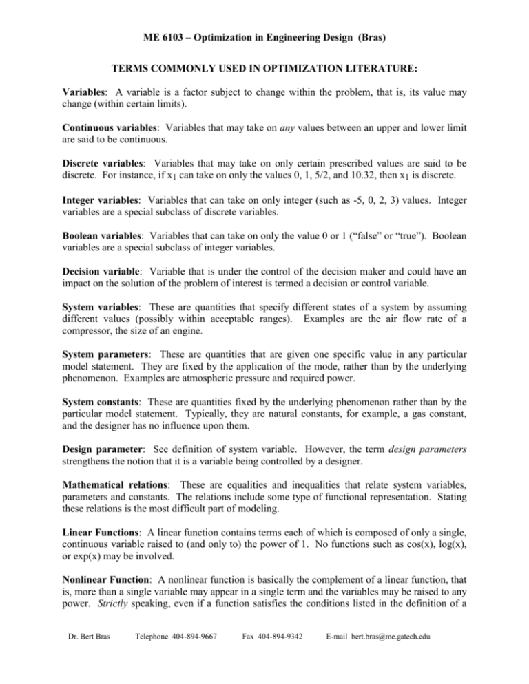
ME 6103 – Optimization in Engineering Design (Bras)
TERMS COMMONLY USED IN OPTIMIZATION LITERATURE:
Variables: A variable is a factor subject to change within the problem, that is, its value may
change (within certain limits).
Continuous variables: Variables that may take on any values between an upper and lower limit
are said to be continuous.
Discrete variables: Variables that may take on only certain prescribed values are said to be
discrete. For instance, if x1 can take on only the values 0, 1, 5/2, and 10.32, then x1 is discrete.
Integer variables: Variables that can take on only integer (such as -5, 0, 2, 3) values. Integer
variables are a special subclass of discrete variables.
Boolean variables: Variables that can take on only the value 0 or 1 (“false” or “true”). Boolean
variables are a special subclass of integer variables.
Decision variable: Variable that is under the control of the decision maker and could have an
impact on the solution of the problem of interest is termed a decision or control variable.
System variables: These are quantities that specify different states of a system by assuming
different values (possibly within acceptable ranges). Examples are the air flow rate of a
compressor, the size of an engine.
System parameters: These are quantities that are given one specific value in any particular
model statement. They are fixed by the application of the mode, rather than by the underlying
phenomenon. Examples are atmospheric pressure and required power.
System constants: These are quantities fixed by the underlying phenomenon rather than by the
particular model statement. Typically, they are natural constants, for example, a gas constant,
and the designer has no influence upon them.
Design parameter: See definition of system variable. However, the term design parameters
strengthens the notion that it is a variable being controlled by a designer.
Mathematical relations: These are equalities and inequalities that relate system variables,
parameters and constants. The relations include some type of functional representation. Stating
these relations is the most difficult part of modeling.
Linear Functions: A linear function contains terms each of which is composed of only a single,
continuous variable raised to (and only to) the power of 1. No functions such as cos(x), log(x),
or exp(x) may be involved.
Nonlinear Function: A nonlinear function is basically the complement of a linear function, that
is, more than a single variable may appear in a single term and the variables may be raised to any
power. Strictly speaking, even if a function satisfies the conditions listed in the definition of a
Dr. Bert Bras
Telephone 404-894-9667
Fax 404-894-9342
E-mail bert.bras@me.gatech.edu
ME 6103 – Optimization in Engineering Design (Bras)
linear function, it is not considered linear if any of the variables involved are discrete. However,
it is common practice to term such a function a linear discrete (or integer) function.
Mathematical model: A mathematical model consists of a set of related mathematical functions
whose purpose is to simulate the response of the system being modeled. A linear mathematical
model consists of solely linear functions; a nonlinear mathematical model involves one or more
nonlinear functions.
Equation: A mathematical equation, represented in general as f(x) = b (i.e., some function of the
variables x = x1, x2, ..., xn is equal to a constant right-hand side value, b) expresses the
equivalence between the function on the left and the function on the right.
Inequalities: Consider the previous definition. If the function on the left can equal or exceed
the function or constant on the right, then this is called an inequality and, more specifically, a
type II inequality. On the other hand, if the function on the left can be less than or equal to the
function or constant on the right, then this is called a type I inequality. Mathematically, they are
represented as:
f(x)≤b
(type I)
f(x)≥b
(type II)
Objectives: Objectives are represented by mathematical functions of the system variables. Such
functions usually represent the desires of the decision maker/designer – such as to maximize
profit or minimize cost. Objective functions may be linear or nonlinear in form. It is important
to note that the right hand side (RHS) of an objective function (i.e., its value) is left unspecified.
That is, the two most typical forms of objective functions are:
maximize f(x) or
minimize f(x)
Goals: A goal is a mathematical function of the system variables which represents the
combination of an objective with a target (i.e., right-hand-side) value. For example, if we say we
wish to maximize profit, that is an objective. However, if we wish to achieve a profit level of at
least, say, $1,000, we have established a goal. Notice in particular that, given a target value, any
objective may be converted into a goal. The mathematical form of a goal is either
f(x) ≤ b
or
f(x) ≥ b
or
f(x) = b
depending upon the situation.
Constraints: A constraint has the same mathematical appearance as a goal (i.e., it is either a
type I or type II inequality or an equality). However, the difference between a goal and a
constraint is that a goal implies some flexibility, whereas a constraint, at least in the
mathematical sense, is absolute or inflexible. A solution is called feasible if no constraints are
violated and infeasible if one or more constraints are violated.
Dr. Bert Bras
Telephone 404-894-9667
Fax 404-894-9342
E-mail bert.bras@me.gatech.edu