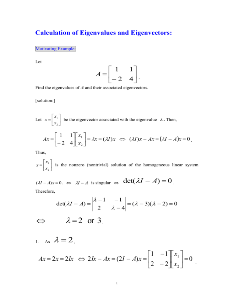
Calculation of Eigenvalues and Eigenvectors:
Motivating Example:
Let
 1
A
 2
1
4 .
Find the eigenvalues of A and their associated eigenvectors.
[solution:]
x 
Let x   1  be the eigenvector associated with the eigenvalue  . Then,
 x2 
 1 1  x1 
Ax  
  x   x  (I ) x  (I ) x  Ax  I  Ax  0 .

2
4

 2 
Thus,
x 
x   1  is the nonzero (nontrivial) solution of the homogeneous linear system
 x2 
(I  A) x  0 .  I  A is singular 
det( I  A)  0 .
Therefore,
det( I  A) 

1.
As
 1
2
1
 (  3)(  2)  0
4
  2 or 3 .
  2,
1  1  x1 
Ax  2 x  2Ix  2Ix  Ax  (2I  A) x  
x   0
2

2

 2 
1
.

 x1  1
x      t , t  R.
 x2  1
1
  t , t  0, t  R, are the eigenvecto rs
1
associated with   2
2.
As
  3,
2  1  x1 
Ax  3x  3Ix  3Ix  Ax  (3I  A) x  
0



2  1  x2 

.
 x1  1 / 2
x       r , r  R.
 x2   1 
1 / 2
   r , r  0, r  R, are the eigenvecto rs
 1 
associated with   3
Note:
In the above example, the eigenvalues of A satisfy the following equation
det( I  A)  0 .
After finding the eigenvalues, we can further solve the associated homogeneous
system to find the eigenvectors.
2
Definition of the characteristic polynomial:
Let
  . The determinant
Ann  a ij
  a11  a12
 a 21   a 22
f ( )  det( I  A) 


 a n1
 an2


 a1n
 a 2n


   a nn
,
is called the characteristic polynomial of A.
f ( )  det( I  A)  0 ,
is called the characteristic equation of A.
Theorem:
A is singular if and only if 0 is an eigenvalue of A.
[proof:]
: .
A is singular  Ax  0 has non-trivial solution  There exists a nonzero vector
x such that
Ax  0  0 x .
 x is the eigenvector of A associated with eigenvalue 0.
:
0 is an eigenvalue of A  There exists a nonzero vector x such that
Ax  0  0 x .
 The homogeneous system Ax  0 has nontrivial (nonzero) solution.
 A is singular.
3
Theorem:
The eigenvalues of A are the real roots of the characteristic polynomial
of A.
:
Let  * be an eigenvalue of A associated with eigenvector u. Also, let f ( ) be the
characteristic polynomial of A. Then,
Au  * u  * u  Au  * Iu  Au  (* I  A)u  0  The homogeneous system
has nontrivial (nonzero) solution x  * I  A is singular 
det(* I  A)  f (* )  0 .
  * is a real root of f ( )  0 .
:
Let  r be a real root of f ( )  0  f (r )  det(r I  A)  0  r I  A is a
singular matrix  There exists a nonzero vector (nontrivial solution) v such that
(r I  A)v  0  Av  r v .
 v is the eigenvector of A associated with the eigenvalue  r .
Procedure of finding the eigenvalues and eigenvectors of A:
1. Solve for the real roots of the characteristic equation
f ( )  0 . These
real roots 1 , 2 , are the eigenvalues of A.
2. Solve for the homogeneous system
 A  i I x  0
or
i I  Ax  0 ,
i  1,2,  . The nontrivial (nonzero) solutions are the eigenvectors associated with
the eigenvalues
i .
4
Example:
Find the eigenvalues and eigenvectors of the matrix
5
A
4

2
4
5
2
2
2
.
2

[solution:]
 5
f ( )  det( I  A)   4
2
4
 5
2
2
 2    1   10  0
 2
2
   1, 1, and 10.
1. As
 1,
 4
1  I  Ax   4
 2
4
4
2
 2  x1 
 2  x 2   0 .
 1  x3 
 x1   s  t   1  1
 x1  s  t , x2  s, x3  2t  x   x2    s   s  1   t  0 , s, t  R.
 x3   2t   0   2 
Thus,
 1  1
s  1   t  0 , s, t  R, s  0 or t  0 ,
 0   2 
are the eigenvectors associated with eigenvalue
2. As
  10 ,
5
 1.
4
 5
10  I  Ax   4
 2
5
2
 2  x1 
 2  x2   0 .
8   x3 
 x1  2r  2
 x1  2r , x2  2r , x3  r  x   x2   2r   r 2, r  R.
 x3   r  1
Thus,
 2
r 2, r  R, r  0 ,
1
are the eigenvectors associated with eigenvalue
  10 .
Example:
0
A  2
0
1
3
4
2
0 .
5
Find the eigenvalues and the eigenvectors of A.
[solution:]

1
2
f ( )  det(I  A)   2   3
0    1   6  0
0
4  5
2
   1, 1, and 6.
3. As
 1,
 1 1
 A  1  I x   2 2
 0 4
6
2  x1 
0  x2   0 .
4  x3 
 x1   1 
 x   x2   t  1, t  R.
 x3   1 
Thus,
1
t  1, t  R, t  0 ,
 1 
are the eigenvectors associated with eigenvalue
4. As
 1.
  6,
 6
 A  6  I x   2
 0
1
3
4
2   x1 
0   x2   0 .
 1  x3 
 x1  3
x   x2   r 2, r  R.
 x3  8
Thus,
 3
r 2, r  R, r  0 ,
8
are the eigenvectors associated with eigenvalue
  6.
Note:
In the above example, there are at most 2 linearly independent
eigenvectors
 3
r 2, r  R, r  0
8
and
matrix A.
7
1
t  1, t  R, t  0
 1 
for
3 3
The following theorem and corollary about the independence of the
eigenvectors:
Theorem:
Let
u1 , u 2 ,, u k
be the eigenvectors of a n  n matrix A associated
with distinct eigenvalues
u1 , u 2 ,, u k
1 , 2 ,, k
, respectively, k  n . Then,
are linearly independent.
[proof:]
Assume
u1 , u 2 ,, u k
are linearly dependent. Then, suppose the
dimension of the vector space V generated by
u1 , u 2 ,, u k

k


i 1

is j  k
(i.e. the dimension of V  u | u   ci ui , ci  R, i  1,2,, k   the vector
space generated by
vectors of
u1 , u 2 ,, u k ).
u1 , u 2 ,, u k
generality, let
u1 , u2 ,, u j
generate V (i.e.,
which also generate V. Without loss of
be the j linearly independent vectors which
u1 , u2 ,, u j
is a basis of V). Thus,
u j 1 
ai ' s
There exists j linearly independent
j
a u
i 1
i
i ,
are some real numbers. Then,
Au j 1
j
j
 j

 A  ai ui    ai Aui   ai i ui
i 1
 i 1
 i 1
8
Also,
j
j
i 1
i 1
Au j 1   j 1u j 1   j 1  ai ui   ai  j 1ui
Thus,
j
j
a  u  a 
i 1
Since
i
i
i
u1 , u2 ,, u j
i 1
i
u 
j 1 i
 a 
j
i 1
i
i
  j 1 ui  0 .
are linearly independent,
a1  j 1  1   a 2  j 1  2     a j  j 1   j   0 .
Futhermore,
1 , 2 ,,  j
are distinct,  j 1  1  0,  j 1  2  0,,  j 1   j  0
j
 a1  a 2    a j  0  u j 1   ai ui  0
i 1
It is contradictory!!
Corollary:
If a n  n matrix A has n distinct eigenvalues, then A has n linearly
independent eigenvectors.
9