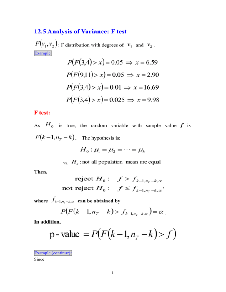
12.5 Analysis of Variance: F test
F v1 ,v2  : F distribution with degrees of v1
and v2 .
Example:
PF 3,4  x  0.05  x  6.59
PF 9,11  x  0.05  x  2.90
PF 3,4  x  0.01  x  16.69
PF 3,4  x  0.025  x  9.98
F test:
As
H 0 is true, the random variable with sample value f is
F k  1, nT  k  . The hypothesis is:
H 0 : 1  2    k
vs.
H a : not all population mean are equal
Then,
f  f k 1, nT  k ,
reject H 0 :
f  f k 1, nT  k , ,
not reject H 0 :
where
f k 1,nT k ,
can be obtained by


P F k  1, nT  k   f k 1, nT  k ,   .
In addition,
p - value  PF k 1, nT  k   f 
Example (continue):
Since
1
MSB
f 

MSW
ns X2
 9  f k 1, nT  k ,  f 2,15,0.05  3.68
3
 n  1s
i 1
2
i
i
,
n3
where


P F k  1, nT  k   f k 1,nT k ,  PF 2,15  f 2,15,0.05   0.05  f 2,15,0.05  3.68
Therefore, we reject
H 0 . In addition,
p  value  PF k  1, nT  k   f   PF 2,15  9  0.0027  0.05  
H0 .
we also reject
Example:
The following data are the number of products of 3 different production lines.
Number of Products
210
215
205
180
160
195
145
170
165
Line 1
Line 2
Line 3
Let
1 ,  2
and
3
180
190
160
175
170
155
190
155
175
be the mean number of products of the 3 production
lines. Please test the hypothesis
H 0 : 1   2   3
with
  0.05 .
[solution:]
n1  n2  n3  6, nT  n1  n2  n3  18 .
and
x1  195.83, x2  175, x3  161.6, x  177.5.
Then,
 n x
k
MSB 
j 1
j
 x
2
j
k 1
6  195.8  177.5  6  175  177.5  6  161.6  177.5

 1779.4 a
3 1
2
2
nd
2
2
 n  1s  x
k
MSW 

k
2
j
j
j 1
nT  k

nj
j 1 i 1
 xj 
2
j ,i
nT  k
210  195.82    190  195.82  180  1752    155  1752  145  161.62    175  161.62
18  3
 216.91
Therefore,
MSB
1779.4

 8.2  3.68  f 2,15, 0.05  f k 1,nT k , ,
MSW
216.91
f 
H0 .
we reject
Example:
The following ANOVA table for 4 normal populations with the same variance  2
1 ,  2 ,  3 ,  4 .
and means
Source
Sum of
Square
Degree of
Freedom
Mean Square
F
Between
(1)
(3)
237.4
(6)
Within
(2)
(4)
(5)
Total
1909.22
22
(a) Please complete the above ANOVA table.
(b) Test
H 0 : 1  2  3  4
at   0.05 .
[solution:]
(a)
k  4 , (3)  k  1  4  1  3 , (4)  22  (3)  22  3  19 .
(1)
(1)

 (1)  237.4  3  712.22
(3)
3
( 2)  1909.22  (1)  1909.22  712.22  1197
237.4 
( 2) 1197

 63
( 4)
19
237.4 237.4
(6) 

 3.767
(5)
63
(5) 
3
Therefore, ANOVA table is
Source
Sum of
Square
Degree of
Freedom
Mean Square
F
Between
712.22
3
237.4
3.767
Within
1197
19
63
Total
1909.22
22
(b)
f  3.767  3.13  f 3,19, 0.05  f k 1,nT k , .
Online Exercise:
Exercise 12.5.1
Exercise 12.5.2
4