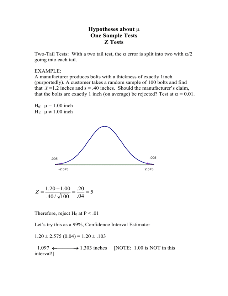
Hypotheses about 
One Sample Tests
Z Tests
Two-Tail Tests: With a two tail test, the  error is split into two with /2
going into each tail.
EXAMPLE:
A manufacturer produces bolts with a thickness of exactly 1inch
(purportedly). A customer takes a random sample of 100 bolts and find
that X =1.2 inches and s = .40 inches. Should the manufacturer’s claim,
that the bolts are exactly 1 inch (on average) be rejected? Test at  = 0.01.
H0:  = 1.00 inch
H1:   1.00 inch
.005
.005
-2.575
Z
2.575
1.20  1.00 .20

5
.40 / 100 .04
Therefore, reject H0 at P < .01
Let’s try this as a 99%, Confidence Interval Estimator
1.20  2.575 (0.04) = 1.20  .103
1.097 ——— 1.303 inches
interval!]
[NOTE: 1.00 is NOT in this
EXAMPLE:
A toothpick manufacturer wants every box to contain exactly (on average)
500 toothpicks. Suppose you took a random sample of n = 81 boxes, and
found:
X =498 toothpicks
S = 9 toothpicks
Test at = .10
H0:  = 500
H1:   500
.05
.05
-1.645
Z
498  500  2

 2
9
1
81
1.645
REJECT H0
Therefore, we reject H0 at p < .1
As a 90%, Confidence Interval:
 9 
 = 498  1.645(1)
 81 
498  1.645 
496.36 ——— 499.65 toothpicks per box
[REJECT H0 : 500 is NOT in the interval]
EXAMPLE:
A researcher claims that 10 year olds watch 6.6 hours of TV daily. You
try to verify this with the following sample data.
n=100
X =6.1 hours
S = 2.5 hours
Test at = .01
H0:  = 6.6
H1:   6.6
.005
.005
-2.575
Z
2.575
6.1  6.6  .50

 2
2.5
.25
100
DO NOT REJECT H0
Therefore, we do not reject H0 at p < .01
As a 99%, Confidence Interval Estimate:
6.1  2.575
2.5
100
= 6.1  2.575(.25) = 6.1  .644
5.456 hours ——— 6.744 hours
Since μ0 = 6.1 IS covered by this CIE, we do not reject H0
EXAMPLE:
A company wishes to determine if the average salary of its clerks is really
$340. The company researcher takes a sample of 64 clerks and finds that
X =$300 and s = $80. Test at  = 0.05.
H0:  = $340
H1:   $340
2.5%
2.5%
1.96
-1.96
Z
300  340  40

 4
10
80 / 64
REJECT H0
Therefore, reject H0 at p < .05
As a 95%, CIE:
300 
80
64
= 300  1.96(10) = 300  19.6
$280.40 ——— $319.60
[NOTE: 340 is not in this interval.]
One-Tail Tests
In previous examples, the tests of hypothesis were of the two-tailed
variety. That is, the rejection region was divided equally into both tails of
the sampling distribution of the statistic.

/2
Sometimes we are interested in testing hypotheses that are to be rejected
only if the sample shows significant deviation in one direction. In these
cases deviations in the other direction only confirm the hypothesis.
For example, in testing the life of ball bearings, the buyer wants  ≥ 300 days and will
only reject if < 300 days.
H0:  ≥ 300 days
H1:  < 300 days
5%
rejection region
[In this course, we will continue to
do all confidence intervals as twosided 2-tail CIEs.]
EXAMPLE:
A manufacturer purchases bulbs that are supposed to burn for a mean life
of at least 3,000 hours, with a standard deviation of 500 hours. A sample
of 100 bulbs is taken, with:
X = 2,800 hours
Test at = .05
H0:  ≥ 3,000 hours
H1:  < 3,000 hours
5%
-1.645
Z
2800  3000  200

 4
50
500 / 100
REJECT H0
Therefore, we reject H0 at p < .05
Using above data, we could construct a 2-sided 95%
Confidence Interval Estimate: 2800  1.96(50)
2702 hours ↔ 2898 hours
EXAMPLE:
A company claims that its weight-reducing drug will cause a weight loss
of at least 10 pounds within one month. A random sample of 64 subjects
is taken and the average weight loss is 7 lbs. with s = 4 lbs.
Test at = .01
H0:  ≥ 10
H1:  < 10
.01
-2.33
Z
7  10
3

 6
.5
4 / 64
Therefore, reject H0 at p < .01
REJECT H0
EXAMPLE:
The FTC wishes to determine whether 9 oz candy bars really are 9 oz.
They take a sample of 49 candy bars:
X = 8.94 oz
S = .12 oz
Test at = .01 level
H0:  ≥ 9 oz
H1:  < 9 oz
.01
-2.33
Z
8.94  9.00  .060

 3.5
.017
.12 / 49
Therefore, reject H0 p < .05
REJECT H0
EXAMPLE:
A wine manufacturer claims that his wine has at most 9 ppm (parts per
million) impurities in a barrel of wine.
Test at = .01
n=64
X = 9.06 ppm impurities
s = 0.12 ppm
H0:  ≤ 9 ppm
H1:  > 9 ppm
.01
+2.33
Z
9.06  9.00
.12 / 64

.060
4
.015
Therefore, reject H0 p < .01
REJECT H0
EXAMPLE:
A company claims that its batteries have a life of at least 100 hours. You
sample:
n=121
X = 97 hours
s = 3 hours
Test at = .05 level
H0:  ≥ 100 hours
H1:  < 100 hours
5%
-1.645
Z
97  100
3

 11
3 / 121 3 / 11
Therefore, reject H0 p < .05
REJECT H0
EXAMPLE:
A company claims that its toasters have an average life of at least 10
years. Use the following sample to test at  = .02.
n=100
X = 9.4 years
s = 1.2 years
H0:  ≥ 10 years
H1:  < 10 years
2%
-2.05
Z
9.4  10
 .60

 5
.12
1.2 / 100
Therefore, reject H0 at p < .02
REJECT H0
The Evian Pure Water Company claims that there are at most 1 ppm units
of urine in its highly overpriced (er, regarded) water. Use the following
sample data to test at α = .05.
n=121 bottles
X = 1.1 ppm
s = .33 ppm
H0:  ≤ 1 ppm
H1:  > 1 ppm
.05
1.645
Z=
1.1  1.0 .10

= 3.3
.33
.03
121
REJECT H0 p < .05
About p-value
What is the “p-value”? It is the probability that we get the data value we
got (the X , as converted to a Zcalc), or worse. We can get that probability
from the Z table. In this case, What is the probability of getting a Zcalc
value of 3.3 or higher (more extreme)?
p=.00048
3.3
p = .5 - .49952 = .00048
This is <.05 (the “nominal” α level).
p-value for a two-tailed test:
then we want the probability of getting the Zcalc from the data or worse
(symmetrically, on both sides of the distribution). For example, suppose
we got a Zcalc = -3.
.00135
.00135
-3.0
3.0
p = .00135 + .00135 = .00270
that’s p < .05 (if α is .05) and even p < .01 (if α is .01)
EXAMPLE:
A manufacturer produces drill bits with an intended life of at least 580
hours and a standard deviation of 30 hours. A quality control scientist
draws a sample of 100 bits and finds X =577. Test at α=.05 to see if the
machinery needs adjusting.
H0:  ≥ 580 hours
H1:  < 580 hours
5%
-1.645
Z=
577  580  3

= -1.00
30
3
100
DO NOT REJECT H0
P > .05
Do NOT adjust the machinery.