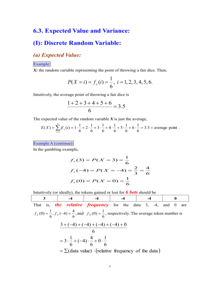
6.3. Expected Value and Variance:
(I): Discrete Random Variable:
(a) Expected Value:
Example:
X: the random variable representing the point of throwing a fair dice. Then,
1
P( X  i )  f x (i)  , i  1, 2, 3, 4, 5, 6.
6
Intuitively, the average point of throwing a fair dice is
1 2  3  4  5  6
 3.5 .
6
The expected value of the random variable X is just the average,
6
E ( X )   if x (i )  1 
i 1
1
1
1
1
1
1
 2   3   4   5   6   3.5  average point .
6
6
6
6
6
6
Example A (continue):
In the gambling example,
f x (3)  P ( X  3) 
1
6
f x ( 4)  P ( X  4) 
f x (0)  P ( X  0) 
2
4

3
6
1
6
Intuitively (or ideally), the tokens gained or lost for 6 bets should be
3
-4
-4
-4
-4
0
is, the relative frequency for the data 3, -4, and 0 are
1
4
1
f X (0)  , f X (4)  , and f X (0)  , respectively. The average token number is
6
6
6
That
3  (4)  (4)  (4)  (4)  0
6
1
4
1
 3   (4)   0 
6
6
6
 (data value)  relative frequency of the data 
1
Since the relative frequency plays the role of the probability distribution,
while the the values of the random variable plays the role of the data values,
it is sensible to define the expected value of the random variable X by
E( X )
 3  f x (3)  (4)  f x (4)  0  f x (0)
1
2
1  13
.
 3   (4)   0  
6
3
6
6
 the value of the random variable   the probabilit y of the value 
Therefore, on the average, the gambler will lose
 13
for every bet.
6
Similarly, the expected value of the random variable Y is
E (Y )  30  f y (30)  (40)  f y (40)  0  f y (0)  30 
1
2
1  130
 (40)   0  
.
6
3
6
6
Formula for the expected value of a discrete random
variable:
Let a1 , a2 ,, an , be all the possible values of the discrete random
variable X and
f (x)
is the probability distribution. Then, the
expected value of the discrete random variable X is
E ( X )     ai f (ai )  a1 f (a1 )  a2 f (a2 )    an f (an )  
i
Note: As the grouped data available are
a1 , a2 ,, an
with frequencies
F1 , F2 ,, Fn , respectively, i.e., with relative frequencies
f a1  
F
F1
F
, f a2   2 ,  , f a1   n ,
N
N
N
the average of the data is
2
a1 F1  a2 F2    an Fn
N
F
F
F
 a1  1  a2  2    an  n
N
N
N
 a1 f (a1 )  a2 f (a2 )    an f (an )
n
where
F
i 1
i
N
(b) Variance:
Example:
Suppose we want to measure the variation of the random variable X in the dice
example. Then, the square distance between the values of X and its mean E(X)=3.5
can be used, i.e., (1  3.5) 2 , (2  3.5) 2 , (3  3.5) 2 , (4  3.5) 2 , (5  3.5) 2 , (6 - 3.5) 2 can
be used. The average square distance is
(1  3.5) 2  (2  3.5) 2  (3  3.5) 2  (4  3.5) 2  (5  3.5) 2  (6  3.5) 2 8.75

.
6
3
Intuitively, large average square distance implies the values of X scatter widely.
The variance of the random variable X is just the average square distance (the
expected value of the square distance). The variance for the dice example is
6
Var ( X )  EX  E ( X )  E ( X  3.5) 2   (i  3.5) 2 f (i )
2
i 1
1
1
1
1
1
1
 (1  3.5) 2   (2  3.5) 2   (3  3.5) 2   (4  3.5) 2   (5  3.5)   (6  3.5) 2 
6
6
6
6
6
6
8.75

 the average square distance
3
Example A (continue):
Intuitively (or ideally), the tokens gained or lost for 6 bets should be
3
-4
-4
-4
-4
0
is, the relative frequency for the data 3, -4, and 0
1
4
1
f X (0)  , f X (4)  , and f X (0)  , respectively. The average of the data is
6
6
6
That
3
are

 13
. Therefore, the variance for the data, considered as the population, is
6
3   2  (4   ) 2  (4   ) 2  (4   ) 2  (4   ) 2  0   2
6
4
2 1
2 1
 3      (4   ) 2   0    
6
6
6
 ( the square of the deviation)  relative frequency of the data 
Since the relative frequency plays the role of the probability distribution,
while the the values of the random variable plays the role of the data values,
it is sensible to define the variance of the random variable X by
Var ( X )
2
2
2
   13 

   13 
  13 
 3  
  f x (3)   4  
  f x (4)  0  
   f x ( 0)
 6 
  6 

  6 
 31  1   11  2  13  1
   
       7.472
 6 6  6  3 6 6
 the square of the deviation of the value of the random variable  
the probabilit y of the value 
2
2
2
.
Similarly, the variance of the random variable Y is
2
2
2


   130 
  130 
  130 
Var (Y )  30  
  f y (30)   40  
  f y (40)  0  
  f y (0)
 6 
 6 


  6 
 310  1   110  2  130  1

  
  
   747.2
 6  6  6  3  6  6
2
2
2
Formula for the variance of a discrete random variable:
Let a1 , a2 ,, an , be all the possible values of the discrete random
variable X and
f (x)
is the probability distribution. Let   E (X )
be the expected value of X. Then, the variance of the discrete random
variable X is
4
Var ( X )   2  EX  E ( X )   (ai   ) 2 f (ai )
2
i
 (a1   ) 2 f (a1 )  (a2   ) 2 f (a2 )    (an   ) 2 f (an )  
Note: As the grouped data available are
a1 , a2 ,, an
with frequencies
F1 , F2 ,, Fn , respectively, i.e., with relative frequencies
f a1  
F
F1
F
, f a2   2 ,  , f a1   n ,
N
N
N
the variance of the data, considered as the population, is
a1   2 F1  a2   2 F2    an   2 Fn
N
 a1    
F1
2 F
2 F
 a2     2    an     n
N
N
N
2
2
2
 a1    f (a1 )  a2    f (a2 )    an    f (an )
2
n
where
F
i 1
i
N
Example 1:
The probability distribution function for a discrete random variable X is
f ( x )  2k , x  1
3k , x  3
4k , x  5
0, otherwise
where k is some constant. Please find
(a) k. (b) P( X  2) (c) E ( X ) and Var( X )
[solution:]
(a)
 f ( x)  f (1)  f (3)  f (5)  2k  3k  4k  9k  1
x
 k 
1
9
.
5
(b)
P( X  2)  P( X  3 or X  5)  P( X  3)  P( X  5)
1 7
.
 f (3)  f (5)  3k  4k  7k  7  
9 9
(c)
u  E ( X )   xf ( x)  1 f (1)  3  f (3)  5  f (5)
x
2
3
4 31
 1  3   5  
9
9
9 9
and
Var ( X )    x  u  f ( x)
2
x
2
2
2
31 
31 
31 



 1 
  f (1)   3 
  f (3)   5 
  f (5)
9 
9 
9 



2

 22  2 16 3 14 2 4 200

 
 
 
81
9
81 9
81 9
81
(II): Continuous Random Variable:
(a) Expected Value:
Example B (continue):
Z: the random variable representing the delay flight time taking values in [0,1].
1
P(0  Z  0.5)  P(0.5  Z  1)  .
2
Then, the probability density function for Z is
f 2 ( x)  1, 0  x  1.
Intuitively, since there is equal chance for any delay time in [0,1], 0.5 hour seems to
be a sensible estimate of the average delay time.
The expected value of the random variable Z is just the average delay time.
1
1
x2
E ( Z )   xf2 ( x)dx   xdx 
2
0
0
6
1
0
 0.5  average delay time .
Formula for the expected value of a continuous random
variable:
Let the continuous random variable X taking values in [a,b] and
f (x)
is the probability density function. Then, the expected value of
the continuous random variable X is
b
E ( X )     xf ( x)dx .
a
Example B (continue):
In the flight time example, suppose the probability density function for Z is
4
2
f1 ( x)  , 0  x  0.5; f1 ( x)  , 0.5  x  1.
3
3
Then, the expected value of the random variable Z is
1
E ( Z )   xf1 ( x)dx 
0
0.5
1
4
2
x2 4
x

dx

x

dx


0 3 0.5 3
2 3
0.5
0

x2 2

2 3
1
0.5
 0.5 2 4 0 2 4   12 2 0.5 2 2  5
 
 
     
 
2 3  12
 2 3 2 3  2 3
Therefore, on the average, the flight time is
.
5
hour.
12
(b) Variance:
Example B (continue):
Suppose we want to measure the variation of the random variable Z in the flight time
example. Suppose f 2 ( x) is the probability density function for Z. Then, the square
distance between the values of Z and its mean E ( Z ) 
2
1
can be used, i.e.,
2
1

 x   , 0  x  1 can be used. The average square distance is
2

7
1
 x3 x2 x  1
 1
 1
E Z      x   f 2 ( x)dx      0
 2 0  2
 3 2 4
2
2
1 1 1 0 0 0 1
         .
 3 2 4   3 2 4  12
The variance of the random variable Z is just the average square distance (the
expected value of the square distance). The variance for the flight time example is
Var ( Z )  E Z  E ( Z )
2
2
1
1

 E Z   
 the average square distance .
2
12

Formula for the variance of a continuous random variable:
Let the continuous random variable X taking values in [a,b] and
f (x)
is the probability distribution. Let   E (X ) be the expected
value of X. Then, the variance of the continuous random variable X is
b
Var ( X )    EX  E ( X )   ( x  u) 2 f ( x)dx
2
2
a
Example B (continue)
In the flight time example, suppose f1 ( x) is the probability density function for Z.
Then, the variance of the random variable Z is
Var ( Z )  E Z  E ( Z )
2
2
2
 x 3 5 x 2 25 x  4

  

12 144  3
 3
0.5
0
0.5
 x 3 5 x 2 25 x  2

  

12 144  3
 3
1
0. 5
1

11
144
Example 2:
The probability density function for a continuous random variable X is
f ( x )  a  bx 2 , 0  x  1
0, otherwise.
where a, b are some constants. Please find
(a) a, b if E ( X ) 
2
5
5 4
5 2



   x   f 1 ( x)dx    x    dx    x    dx
12 
12  3
12  3
0
0
0.5
1
3
(b) Var( X ) .
5
[solution:]
(a)
8
b


a

bx
dx

1

ax

x

3
1

1
f ( x)dx  1 
2
0
| 1
3 1
0
0
b
 a  1
3
and
1
1


a
b
a b 3
E ( X )   xf ( x)dx   x a  bx 2 dx  x 2  x 4 |10   
2
4
2 4 5
0
0
Solve for the two equations, we have
a
3
6
, b
5
5
.
(b)
f ( x) 
3
6 2

x , 0  x 1
5
5
0, otherwise.
Thus,
 3
Var ( X )  EX  E ( X )  E ( X 2 )  E ( X )  E ( X 2 )   
 5
2
2
9
9
3 6 
  x f ( x)dx 
  x 2   x 2 dx 
25 0  5 5 
25
0
1
1
2
1
6
9 1 6
9
2
 x 3  x 5 |10    

5
25
25 5 25 25 25
Example 3:
The probability density function for a continuous random variable X is
x  2

,2 x  4
f ( x)   18

0, otherwise



Please find (a) P X  1 (b) P X 2  9 (c) E X  and Var X 
9
2
[solution:]
(a)
1
 x2 x
x2
 1 1  1 1 2
P X  1  P 1  X  1  
dx             
18
 36 9  1  36 9   36 9  9
1
1
(b)
3
2
3
 x2 x 
x2
x2
25
P X  9  P 3  X  3  
dx   0dx  
dx     
18
18
 36 9  2 36
3
3
2

2

3
(c)
EX    
x  2 dx 
x
4

2
18
4
 x2 x 
 x3 x2 
  18  9 dx   54  18   2 .
 2
2
4
Since
   x
4
EX
2
2
2
x  2 dx 

18
4
 x3 x2 
 x4 x3 
  18  9 dx   72  27   6 ,
 2
2
4
 
Var  X   E  X     E X 2   2  6  2 2  2 .
2
Example 4:
The probability distribution functions (discrete random variable) or probability
density functions (continuous random variable) for a random variable X are
(a)
c exp  6 x , x  0

f ( x )    cx,  1  x  0

0, otherwise

(b)


f x   cx 2 exp  x 3 , x  0
(c)
x
1
f  x   c  , x  0, 1, 2, 
3
10
Find c .
[solution:]
(a)
  cx 2 
  c exp  6 x 
1 cxdx  0 c exp  6 x dx  1   2   
  1
6
0
1
c c
3c  c
3
   1
 1 c 
2 6
6
2

0

0
(b)


 

  c exp  x 3 
1
3
3
0 cx exp  x dx  1  c 0 3 exp  x dx  1   3   1
0
c
  1 c  3
3
 
2
3
 
(c)
x

1
c   1 

x 0  3 
c 
 1 
 1  1 2

  1  3c  1
c 1        1  c
2
 1  1 
 3  3 

3

2
3
Online Exercise:
Exercise 6.3.1
Exercise 6.3.2
11