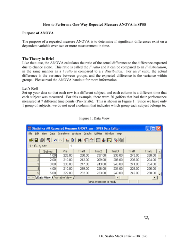
How to Perform a One-Way Repeated Measure ANOVA in SPSS
Purpose of ANOVA
The purpose of a repeated measure ANOVA is to determine if significant differences exist on a
dependent variable over two or more measurement in time.
The Theory in Brief
Like the t-test, the ANOVA calculates the ratio of the actual difference to the difference expected
due to chance alone. This ratio is called the F ratio and it can be compared to an F distribution,
in the same manner as a t ratio is compared to a t distribution. For an F ratio, the actual
difference is the variance between groups, and the expected difference is the variance within
groups. Please read the ANOVA handout for more information.
Let’s Roll
Set-up your data so that each row is a different subject, and each column is a different time that
each subject was measured. For this example, there were 20 golfers that had their performance
measured at 7 different time points (Pre-Trial6). This is shown in Figure 1. Since we have only
1 group of subjects, we do not need a column that indicates which group each subject belongs to.
Figure 1: Data View
Dr. Sasho MacKenzie – HK 396
1
To perform the Repeated Measures ANOVA, select Analyze -> General Linear Model ->
Repeated Measures as shown in Figure 2.
Figure 2: Starting the Repeated Measures ANOVA
Select a name for your within-subject factor. The default is “factor1” but you should change it to
something that has relevance. For our example, change it to “trial”. “Levels” is the number of
times the measure was repeated. In our example, golf drive performance was measured 7 times.
You should then select the “Add” button (See Figure 3).
Figure 3: Selecting the Within-Subject Factor
Dr. Sasho MacKenzie – HK 396
2
After selecting “Add”, the window should look like Figure 4. At this point you could add
another within-subject factor if one existed. “Add” a Measure Name, and hit “Define”.
Figure 4: Measure Name
After you click “Define”, the window shown in Figure 5 should appear. For a 1 Way Repeated
Measure ANOVA, the purpose of this window is to assign each level of the within-subjects
variable to the appropriated column of data. As shown below, the columns Pre, Trial1, and
Trial2 have been assigned. For this example, there are no between-subjects factors.
Dr. Sasho MacKenzie – HK 396
3
Figure 5: The Repeated Measures Window
After assigning each level of the within-subjects variable to a column of data, select the
“Contrasts” button and the Window shown in Figure 6 will appear. Assume that we are
interested in determining if a trial differs significantly from the trial immediately before or the
trial immediately after it. Therefore we would like to conduct a “Repeated” measures contrast.
If it does not say “trials(Repeated)” in the “Factors:” window, then scroll down to find
“Repeated”, and select change. Then hit “Continue”. When we have a variable that increases in
an orderly fashion, such as time, what is most important is the pattern of the means. We are
much more likely to want to be able to make statements of the form "The effect of this drug
increases linearly with dose, " or "This drug is more effective as we increase the dosage up to
some point, and then higher doses are either no more effective, or even less effective." We are
less likely to want to be so specific as to say "The 1 cc dose is less effective that the 2 cc dose,
and the 2 cc dose is less effective than the 3 cc dose. Graduate students often ask me how they
can test an effect such as "Time 2 versus Time 4," and I generally tell them that such a question
is not particularly meaningful when the repeated measure is ordinal. What is probably
happening, and what our eyes say is happening, is that for the Near condition stress levels are
increasing, up to a point, and it is probably of very little interest exactly which levels are
different from which other levels. That is primarily a question of power, and the answer will vary
with the sample size. What is important is that there is some general linear increase, and it is that
on which we will focus. To take a homey example, we all know that children tend to grow taller
as they age. Do you really want a statistical test of whether 9 years olds are taller than 8.75 year
Dr. Sasho MacKenzie – HK 396
4
olds? Statistical significance for such a difference is rarely the point. (Such a test is possible--see
the section on non-ordinal levels--but I just don't think it is usually meaningful.)
Figure 6: Repeated Measures Contrast Window
From the “Repeated Measures” window, select “Plots” and Figure 7 should appear. Select
“trial” and place it in the “Horizontal Axis” box. Following this, the “Add” button will become
selectable. Select “Add” to bring “trials” into the “Plots:” box at the bottom of the window.
Then hit “Continue”.
Figure 7: Plots Window
Dr. Sasho MacKenzie – HK 396
5
From the “Repeated Measures” window, select “Options” and Figure 8 should appear. Check off
“Descriptive statistics” and “Estimates of effect size”. Then hit “Continue”.
Figure 8: Options Window
From the “Repeated Measures” window, select “OK” to run the 1 Way Repeated Measures
ANOVA. The following should help you analyze your data.
The first important, and non-obvious, chart in the SPSS output is the test for sphericity. A
repeated measures ANOVA must meet the assumption of sphericity. Sphericity requires that the
repeated measures demonstrate homogeneity of variance (each group of data has similar
variance) and homogeneity of covariance (the correlation of each repeated measure with the
dependent variable is similar). If the test is significant (which is indicated in Figure 9) then a
correction must be made before the significance of the ANOVA can be interpreted. Three
options for a correction factor are supplied in the last three cells in Figure 9. Each degree of
freedom used to calculate the F ratio is multiplied by the correction factor (Figure 10). This
does not alter the calculated F ratio, but it does increase the probability of making a Type I error.
This is clearly demonstrated by noting the various p-values in Figure 10. In general if the
correction factors are < .75, a correction to F critical should be made.
Dr. Sasho MacKenzie – HK 396
6
Figure 9: Mauchly’s Test of Spericity
b
Ma uchly's Test of Spheri city
Measure: drive
a
Epsilon
W ithin Subject s Effect Mauchly's W
trial
.015
Approx .
Chi-Square
70.385
df
20
Sig.
.000
Greenhous
e-Geis ser
.415
Huynh-Feldt
.483
Lower-bound
.167
Tests the null hypothes is that t he error covariance matrix of the orthonormalized transformed dependent variables is
proportional to an ident ity matrix.
a. May be us ed t o adjust the degrees of freedom for the averaged t ests of s ignificance. Corrected tests are displayed in
the Tests of W ithin-Subject s Effect s table.
b.
Int ercept
FigureDesign:
10 displays
the main results of the one way repeated measure ANOVA. It answers the
W ithin Subject s Design: trial
question; does the dependent variable change significantly across the various trials? Since the
sphericity test was significant, and the correction factors were below .75 (Figure 9), then we
should use the correction. Since all the corrected tests still show p-values < .05, we can say that
there are significant differences in the dependent variable across trials.
Figure 10: Tests of Within-Subjects Effects
Tests of Within-Subjects Effects
Measure: drive
Source
trial
Error(trial)
Sphericity Assumed
Greenhous e-Geisser
Huynh-Feldt
Lower-bound
Sphericity Assumed
Greenhous e-Geisser
Huynh-Feldt
Lower-bound
Type III Sum
of Squares
830.171
830.171
830.171
830.171
3576.400
3576.400
3576.400
3576.400
df
6
2.492
2.899
1.000
114
47.357
55.074
19.000
Mean Square
138.362
333.071
286.399
830.171
31.372
75.520
64.938
188.232
F
4.410
4.410
4.410
4.410
Sig.
.000
.012
.008
.049
Partial Eta
Squared
.188
.188
.188
.188
Figure 11 shows the results of the actions displayed in Figure 6. This table compares each trial
with the adjacent trials. It permits the researcher to determine at which point in time a significant
change in the dependent variables occurs. For example, we can see that at the  = .05 level, the
Pre Trial differs significantly from Trial 1, and Trial 6 differs significantly from Trial 7. With
numerous repeated measures, often this is not as important as identifying a “trend” in the data.
Dr. Sasho MacKenzie – HK 396
7
Figure 11: Tests of Within-Subjects Contrasts
Tests of Within-Subjects Contrasts
Measure: drive
Source
trial
Error(trial)
trial
Level 1 vs. Level 2
Level 2 vs. Level 3
Level 3 vs. Level 4
Level 4 vs. Level 5
Level 5 vs. Level 6
Level 6 vs. Level 7
Level 1 vs. Level 2
Level 2 vs. Level 3
Level 3 vs. Level 4
Level 4 vs. Level 5
Level 5 vs. Level 6
Level 6 vs. Level 7
Type III Sum
of Squares
168.200
68.450
51.200
1.800
92.450
312.050
593.800
324.550
438.800
694.200
434.550
568.950
df
1
1
1
1
1
1
19
19
19
19
19
19
Mean Square
168.200
68.450
51.200
1.800
92.450
312.050
31.253
17.082
23.095
36.537
22.871
29.945
F
5.382
4.007
2.217
.049
4.042
10.421
Sig.
.032
.060
.153
.827
.059
.004
Partial Eta
Squared
.221
.174
.104
.003
.175
.354
Figure 12 shows the plot of the mean scores for each trial, which is probably more valuable then
any of the above statistics. It clearly displays the trend in the data. Performance improved with
the consumption of a few beers, but began to decrease after too many. This is referred to as the
“inverted U”.
Figure 12: Tests of Within-Subjects Contrasts
Estimated Marginal Means of drive
Estimated Marginal Means
228
226
224
222
1
2
3
4
5
6
7
trial
Dr. Sasho MacKenzie – HK 396
8