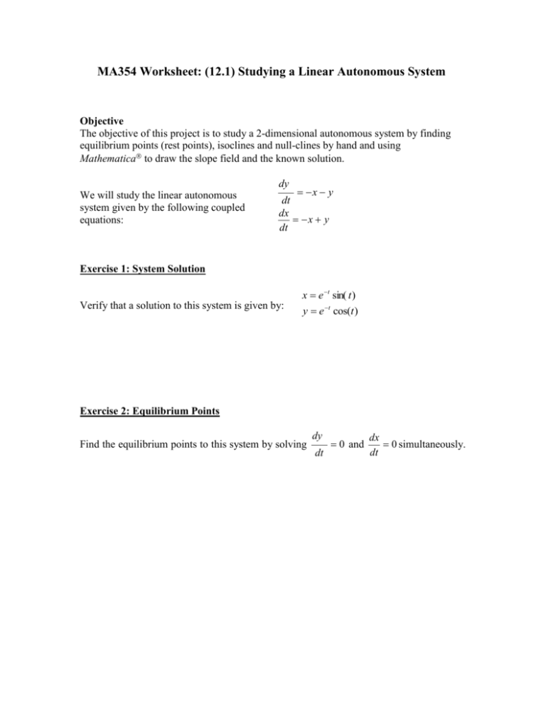
MA354 Worksheet: (12.1) Studying a Linear Autonomous System
Objective
The objective of this project is to study a 2-dimensional autonomous system by finding
equilibrium points (rest points), isoclines and null-clines by hand and using
Mathematica to draw the slope field and the known solution.
dy
We will study the linear autonomous
system given by the following coupled
equations:
 x  y
dt
dx
 x  y
dt
Exercise 1: System Solution
Verify that a solution to this system is given by:
x  e t sin( t )
y  e t cos(t )
Exercise 2: Equilibrium Points
Find the equilibrium points to this system by solving
dy
dt
 0 and
dx
 0 simultaneously.
dt
Exercise 3: Slope field
Use Mathematica to find the slope field, type:
StreamPlot[{-x+y,-x-y},{x,-3,3},{y,-2,2}, AxesTrue]
(a) Sketch the slope field:
(b) Analytically, identify where
dy
dt
quadrant (i.e., x  0 and y  0 ).
and
dx
dt
are positive or negative in the first
(c) Indicate the equilibrium point you identified in Exercise 2 with a filled circle.
Start at a random point in the second quadrant and sketch a trajectory.
Exercise 4: Isoclines and Null-clines
An isocline is a curve in the slope field along which the slope is the same. To find an xdx
isocline, you need to solve need to solve
= c and to find a y-isocline, you need to
dt
dy
solve
= c. As a special case, nullclines occur when c=0.
dt
Nullclines are curves along which the slope field is either completely horizontal
 dy

 dx

= 0  or vertical 
= 0  . A null-cline is a boundary between regions where x' or y'

 dt

 dt

might switch signs. The intersections between x and y null-clines are equilibrium points,
and thus finding null-clines can be a useful way to identify such points.
(a) Find the x- and y-nullclines for the given linear autonomous system.
(b) Confirm that the intersection of the nullclines yields the equilibrium point.
(c) Plot the null-clines on the slope field produced in Mathematica.
Show[
StreamPlot[{-x+y,-x-y},{x,-30,30},{y,20,20},AxesTrue],
Plot[{x,-x},{x,-20,20}]]
Exercise 5: A more generalized linear autonomous system.
Consider the following linear autonomous system:
dy
  Bx  y
dt
dx
  x  By
dt
The solution is given by:
x  e t sin( Bt )
y  e t cos(Bt ) .
(a) Plot the solution for different values of B:
B=1;
x=E^(-t)*Sin[B*t];
y=E^(-t)*Cos[B*t];
ParametricPlot[{x,y},{t,0,10*Pi}, PlotPoints1000,PlotRange1]
Sketch when B=1:
Sketch when B=20:
(b) Find the nullclines as a function of B.
(c) Plotting the solution and the null-clines together, try to estimate which value of B
was used in Fig 12.1, page 469 in your book.
B=1;
x=E^(-t)*Sin[B*t];
y=E^(-t)*Cos[B*t];
Show[ParametricPlot[{x,y},{t,0,10*Pi},
PlotPoints1000,PlotRange1],Plot[{x/B,-x*B},{x,-10,10}]]