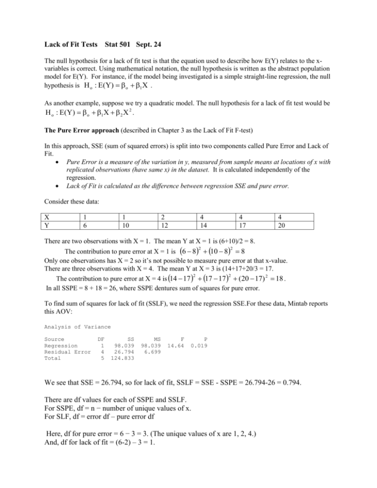
Lack of Fit Tests
Stat 501 Sept. 24
The null hypothesis for a lack of fit test is that the equation used to describe how E(Y) relates to the xvariables is correct. Using mathematical notation, the null hypothesis is written as the abstract population
model for E(Y). For instance, if the model being investigated is a simple straight-line regression, the null
hypothesis is H o : E(Y)   o  1 X .
As another example, suppose we try a quadratic model. The null hypothesis for a lack of fit test would be
H o : E ( Y )   o  1 X   2 X 2 .
The Pure Error approach (described in Chapter 3 as the Lack of Fit F-test)
In this approach, SSE (sum of squared errors) is split into two components called Pure Error and Lack of
Fit.
 Pure Error is a measure of the variation in y, measured from sample means at locations of x with
replicated observations (have same x) in the dataset. It is calculated independently of the
regression.
 Lack of Fit is calculated as the difference between regression SSE and pure error.
Consider these data:
X
Y
1
6
1
10
2
12
4
14
4
17
4
20
There are two observations with X = 1. The mean Y at X = 1 is (6+10)/2 = 8.
The contribution to pure error at X = 1 is 6  8  10  8  8
Only one observations has X = 2 so it’s not possible to measure pure error at that x-value.
There are three observations with X = 4. The mean Y at X = 3 is (14+17+20/3 = 17.
2
2
The contribution to pure error at X = 4 is 14  17   17  17   (20  17) 2  18 .
In all SSPE = 8 + 18 = 26, where SSPE dentures sum of squares for pure error.
2
2
To find sum of squares for lack of fit (SSLF), we need the regression SSE.For these data, Mintab reports
this AOV:
Analysis of Variance
Source
Regression
Residual Error
Total
DF
1
4
5
SS
98.039
26.794
124.833
MS
98.039
6.699
F
14.64
P
0.019
We see that SSE = 26.794, so for lack of fit, SSLF = SSE - SSPE = 26.794-26 = 0.794.
There are df values for each of SSPE and SSLF.
For SSPE, df = n − number of unique values of x.
For SLF, df = error df – pure error df
Here, df for pure error = 6 − 3 = 3. (The unique values of x are 1, 2, 4.)
And, df for lack of fit = (6-2) – 3 = 1.
Defining an MS value as SS/df gives MSPE and MSLF values.
The statistic F = MSLF/MSPE is an F-statistic used to test the null hypothesis. Degrees of
freedom, numerator and denominator, are given by the pure error and lack of fit df’s
respectively.
Here’s the Minitab result for our example.
Source
Regression
Residual Error
Lack of Fit
Pure Error
Total
DF
1
4
1
3
5
SS
98.039
26.794
0.794
26.000
124.833
MS
98.039
6.699
0.794
8.667
F
14.64
P
0.019
0.09
0.782
The SS values for lack of fit and pure error are the values we calculated above. The p-value is p=
0.782 for the F-test of lack of fit. Hence, we do not reject the null hypothesis that the straightline model is correct.
Following is the result we saw in the lab Wednesday for Y = chemical concentration versus X =
time since solution was made. In this case, we reject the straight-line model.
Source
Regression
Residual Error
Lack of Fit
Pure Error
Total
DF
1
13
3
10
14
SS
12.597
2.925
2.767
0.157
15.522
MS
12.597
0.225
0.922
0.016
F
55.99
P
0.000
58.60
0.000
Data Subsetting Approach of Minitab
If n=1 at each unique value of x, pure error cannot be calculated. Minitab offers an alternative
test. It’s hard to find a description of precisely what Minitab does for it’s data subsetting. Here,
though, are the basic ideas.
The null hypothesis is still that the model for E(Y) is correct.
The range of x-values is divided into sub-regions (three I think).
 A model is fit in which the slope is allowed to be different in each region. This
approximates a curved model. The sum of squared errors from this model is used as pure
error sum of squares. The lack of fit SS is, as before, the difference between SSE from
the regression model and the approximate SS for pure error. An approximate F test
comparing lack of fit to pure error is done.
 Also, Minitab only looks at what’s happening in the outer two regions of x. The thinking
is that consequences of using a wrong model are exaggerated in these outer regions.
Following is the result for the tumor size problem done in Wednesday’s lab. The small p-values
indicate we should reject the straight-line model.
Lack of fit test
Possible curvature in variable Time (P-Value = 0.002 )
Possible lack of fit at outer X-values (P-Value = 0.000)
Overall lack of fit test is significant at P = 0.000