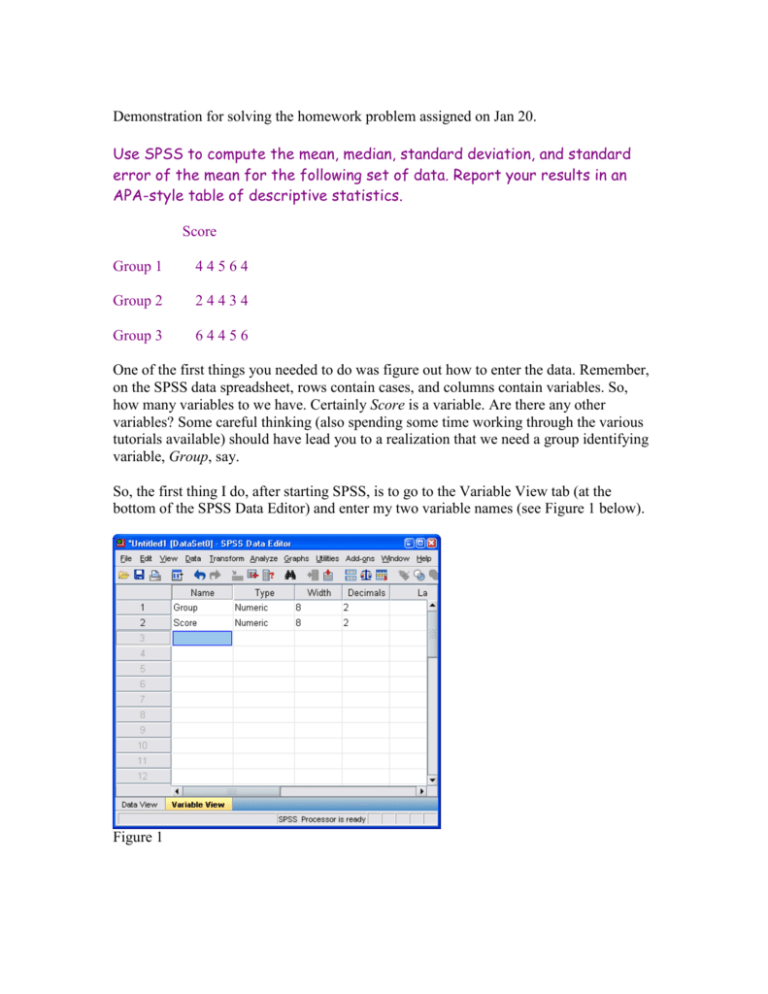
Demonstration for solving the homework problem assigned on Jan 20.
Use SPSS to compute the mean, median, standard deviation, and standard
error of the mean for the following set of data. Report your results in an
APA-style table of descriptive statistics.
Score
Group 1
44564
Group 2
24434
Group 3
64456
One of the first things you needed to do was figure out how to enter the data. Remember,
on the SPSS data spreadsheet, rows contain cases, and columns contain variables. So,
how many variables to we have. Certainly Score is a variable. Are there any other
variables? Some careful thinking (also spending some time working through the various
tutorials available) should have lead you to a realization that we need a group identifying
variable, Group, say.
So, the first thing I do, after starting SPSS, is to go to the Variable View tab (at the
bottom of the SPSS Data Editor) and enter my two variable names (see Figure 1 below).
Figure 1
Next, I switch to the Data View tab and enter the data for each variable (Figure 2).
Everyone in group 1 gets a 1 under Group, those in group 2, get a 2 under group, and so
on. Under score, I enter the scores corresponding to each individual entered under Group.
See the next screen shot.
Figure 2
Now, save the data (to the desktop or somewhere else) before it gets lost.
We want means, medians, standard deviations, and the standard error of the mean for this
set of data. These are all descriptive statistics. Clicking on Analyze opens a dropdown
window showing several analytical procedures. Since we want descriptive statistics, we
clock on Descriptive Statistics, which, in turn, opens another dropdown window (see
Figure 3). There are two procedures in this window that offer promise: Frequencies and
Descriptives. We’ll examine both of these. Click on Frequencies first.
The Frequencies dialog window (Figure 4) opens. Is this the procedure we want? Try it.
The first thing you will notice is that while you can obtain descriptive statistics for the
overall group, there doesn’t seem to be any way of getting the statistics for each
subgroup. You can try the Descriptives procedure next Figure 5. Again, there doesn’t
seem to be any way to compute the statistics we want for each subgroup independently.
So, what to do? The solution is to split the file. In the top menu, click Data > Split. This
opens the Split File window (Figure 6). Click on the Organize output by groups radio
button and move Group into the Groups based on… window and then click OK. The
Figure 3
Figure 4
data file is now split by groups. Any subsequent analysis will be performed separately for
each group. Go back to Analyze > Destructives and click on Frequencies again. Move
Score into the Variables window and click on Statistics and select Mean, Median,
Standard Deviation, and S.E. Mean; and then click Continue (see Figure 6), which
takes you back to the Frequencies window. Click OK.
The Frequencies procedure runs and SPSS produces the output shown following the next
page. For each group, you are given the number of valid scores (N Valid), the number of
missing scores (N Missing) the Mean, Std Error of the Mean, Median, and Standard
Deviation.
A minimal APA-style table of descriptive statistics would look something like the
following:
Ns, Menas, and Standard Deviations
N Mean
Std. Dev.
Group 1
5
4.60
.894
Group 2
5
3.80
1.095
Group 3
5
5.00
1.000
If you wanted to include the median, then it might look something like this:
Descriptive Statistics
N Mean
Group 1
5
4.60
Group 2
5
3.80
Group 3
5
5.00
Median
4.0
4.0
5.0
Std. Dev.
.894
1.095
1.000
Notice the following about the tables: They contain no vertical lines and few horizontal
lines. APA wants nice, clean tables. In most case, use white space to separate rows and
columns. Only the stub headings are separated from the body of the table by a horizontal
line. Also, the standard error of the mean is not given in the tables. This is because the
standard error of the mean, for the sample, is easily computed by:
StdErrM  s X
sX
N
StdDev

N

Which, for Group 1, is
.894
5
.894

2.236
 .400
StdErrM 
If we include the standard error of the mean in our table, it would look like this:
Descriptive Statistics
N
Mean
Group 1
5
4.60
Group 2
5
3.80
Group 3
5
5.00
Median
4.0
4.0
5.0
Std. Dev.
.894
1.095
1.000
Ste Err Mean
.400
.490
.447
Figure 5
Figure 6
Frequencies
Group = 3.00
Statisticsa
Score
N
Valid
5.00000
Missing
Mean
.00000
5.00000
Std. Error of Mean
.44721
Median
5.00000
Std. Deviation
1.00000
a. Group = 3.00
Group = 2.00
N
Valid
5.00000
Missing
Mean
.00000
3.80000
Std. Error of Mean
.48990
Median
4.00000
Std. Deviation
1.09545
a. Group = 2.00
Group = 1.00
Statisticsa
Score
N
Valid
Missing
Mean
Std. Error of Mean
Median
Std. Deviation
a. Group = 1.00
5.00000
.00000
4.60000
.40000
4.00000
.89443