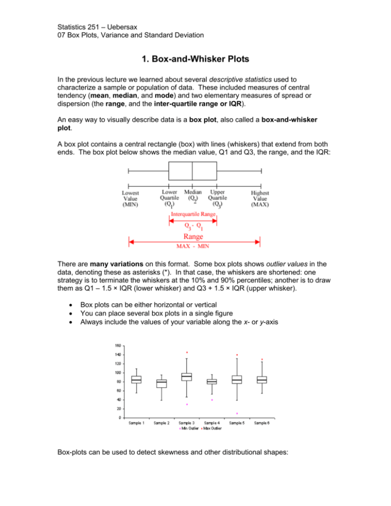
Statistics 251 – Uebersax
07 Box Plots, Variance and Standard Deviation
1. Box-and-Whisker Plots
In the previous lecture we learned about several descriptive statistics used to
characterize a sample or population of data. These included measures of central
tendency (mean, median, and mode) and two elementary measures of spread or
dispersion (the range, and the inter-quartile range or IQR).
An easy way to visually describe data is a box plot, also called a box-and-whisker
plot.
A box plot contains a central rectangle (box) with lines (whiskers) that extend from both
ends. The box plot below shows the median value, Q1 and Q3, the range, and the IQR:
There are many variations on this format. Some box plots shows outlier values in the
data, denoting these as asterisks (*). In that case, the whiskers are shortened: one
strategy is to terminate the whiskers at the 10% and 90% percentiles; another is to draw
them as Q1 – 1.5 × IQR (lower whisker) and Q3 + 1.5 × IQR (upper whisker).



Box plots can be either horizontal or vertical
You can place several box plots in a single figure
Always include the values of your variable along the x- or y-axis
Box-plots can be used to detect skewness and other distributional shapes:
Statistics 251 – Uebersax
07 Box Plots, Variance and Standard Deviation
2. Variance and Standard Deviation
The range and the inter-quartile range (IQR) are relatively primitive measures of the
spread or dispersion of a data set. We'll now discuss the more sophisticated and
commonly used variance and standard deviation. The standard deviation is simply
the square root of the variance.
To motivate our inquiry, suppose we have the following data and want to characterize
the spread of the values:
1, 1, 1, 2, 2, 2, 2, 3, 3, 3, 3, 100
We might choose the range (100 – 1 = 99) to describe the spread. The problem with
that is that 100 is an outlier – most of the data fall between 1 and 3. Simply to describe
the range as 99 is misleading, because it doesn't apply to the bulk of the data.
Using the IQR to summarize range might be a little better, but we could come up with
similar examples to show how it can be misleading.
The problem with the range and the IQR is that both are based only on a subset of the
data: the range considers only two values (the minimum and maximum), and the IQR
only considers half the values (the upper quarter and the lower quarter). What we really
want is a measure of spread that considers all the data values.
So let's try a different approach. One way of operationally defining 'how spread out data
are' is to consider how far individual values are from the mean. So, in the example,
below, suppose the mean is 3.
Statistics 251 – Uebersax
07 Box Plots, Variance and Standard Deviation
In theory, we can calculate the distance of every value from the mean.
And then we might take the average of all these differences from the mean:
1 – 3, 2 – 3, 2 – 3, 0 – 3, 4 – 3, 4 – 3, 5 – 3
Using summation notation, this could be expressed as:
1
N
( x  X )
where N is the number of data values (here N = 7), X is the average value ( X = 3),
and x refers to each of the individual values.
The problem is that we will always have both positive and negative differences, which
will each other out, and we are always left with 0 as the answer!
The way to avoid this is simply to square each difference from the mean. All these
squared differences will be positive. This gives us the formal definitions of the variance
and standard deviation:
variance: the average squared distance from each data value to the mean.
standard deviation: the square root of the variance.
If you remember these simple definitions, you will always be able to correctly calculate
the variance and standard deviation
Applying the first definition to the example above we get the following formula for the
variance:
1
N
(x  X )
2
(x  X )

N
2
Statistics 251 – Uebersax
07 Box Plots, Variance and Standard Deviation
This formula simply means: (1) take the sum, of (2) the squared difference between
each value minus the mean, and (3) divide the sum by N.
There is, however, one minor complication. The formula for the variance is different
depending on whether we are treating the data as a population or as a sample.
Specifically:

If we treat the data as a population, we use the number of observations, N, in the
denominator.

If we treat the data as a sample, we divide by the number of observations minus
1 in the denominator
Population variance and Standard deviation
Sample variance and Standard deviation
In these equations we use a more complete summation notation.
Notice that in the second two equations, we denote the number of cases with a little n,
because we are talking about a sample.
Statistics 251 – Uebersax
07 Box Plots, Variance and Standard Deviation
3. Calculating Variance and Standard Deviation in Excel
Excel has several functions for calculating the variance and standard deviation. You use
different functions, depending on whether you wish to treat your data as a sample or a
population:
Statistic
sample variance
population variance
sample standard deviation
population standard deviation
Excel function
=var(<range>)
=varp(<range>)
=stdev(<range>)
=stdevp(<range>)
where <range> means the range of cells that contain your data, e.g., a:a or a1:a100.
So, for example, if your data are in Column A, the sample variance would be given by
the Excel formula:
=var(a:a)
Reading: pp. 97–106.